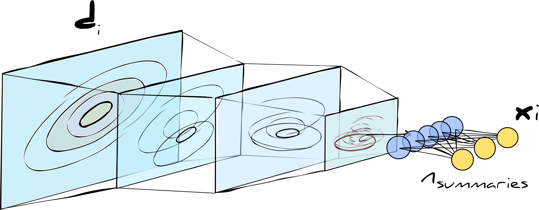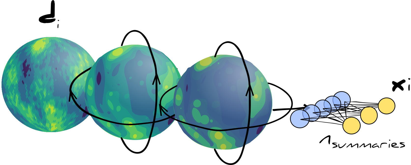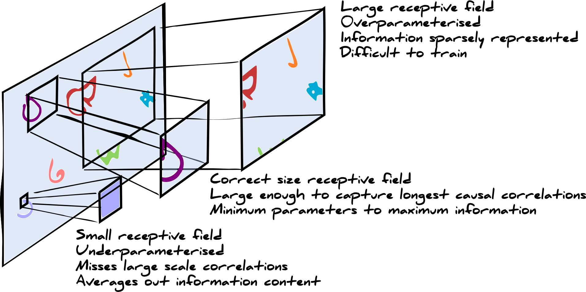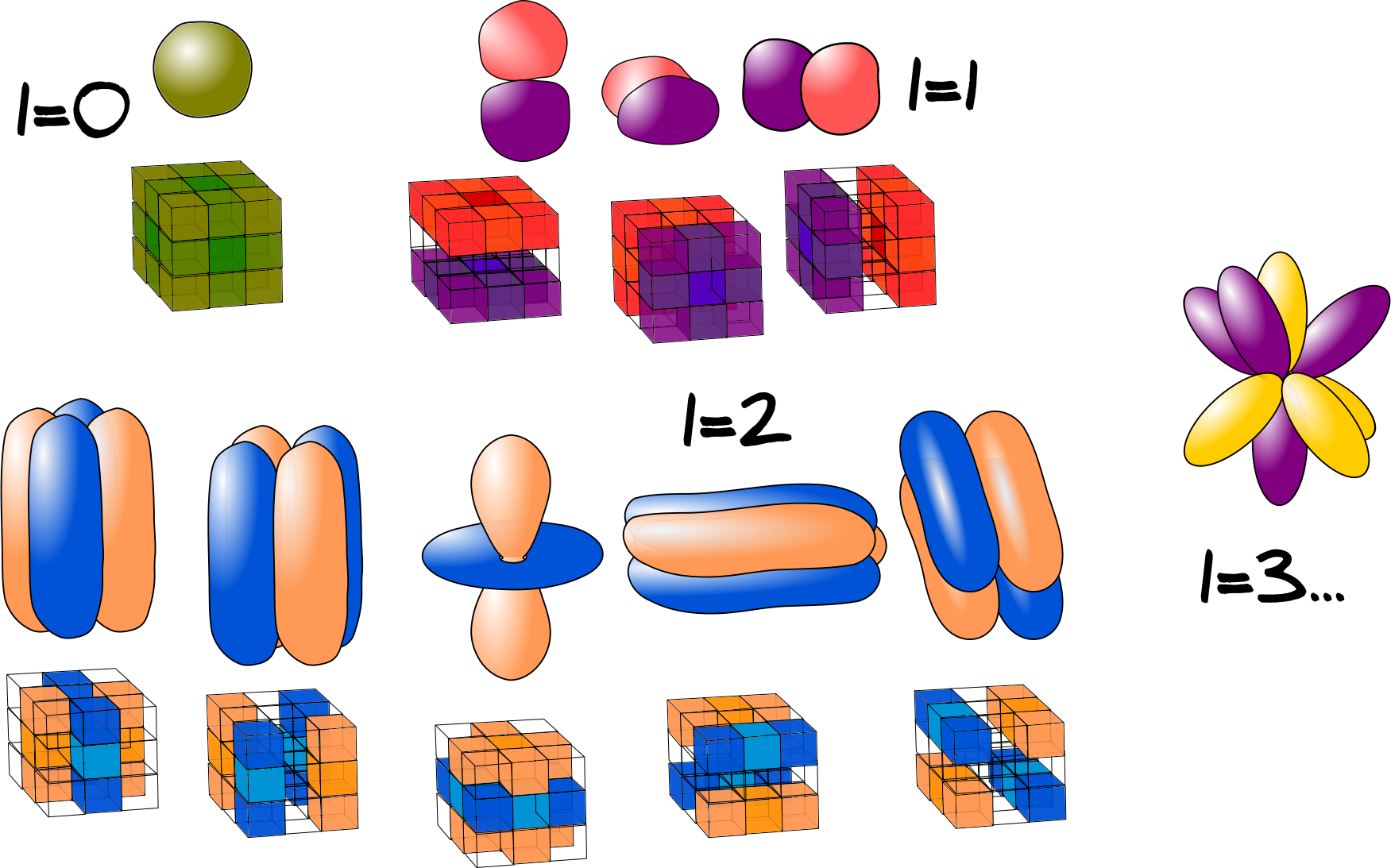


Joint distribution of parameters, $\boldsymbol{\theta}$, and possible data, ${\bf d}$,
which can be generated by a model, $\mathcal{M}:\boldsymbol{\theta}\to{\bf d}$
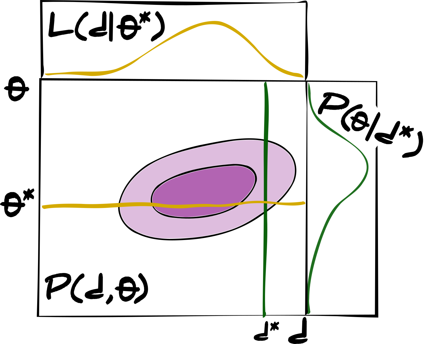
Obligatory Bayes Theorem
Likelihood $$\mathcal{L}({\bf d}|\boldsymbol{\theta}^*,\mathcal{M})$$
Posterior $$\mathcal{P}(\boldsymbol{\theta}|{\bf d}^*,\mathcal{M})$$
Parameter inference using neural networks
It's common to try and predict model parameters by regression
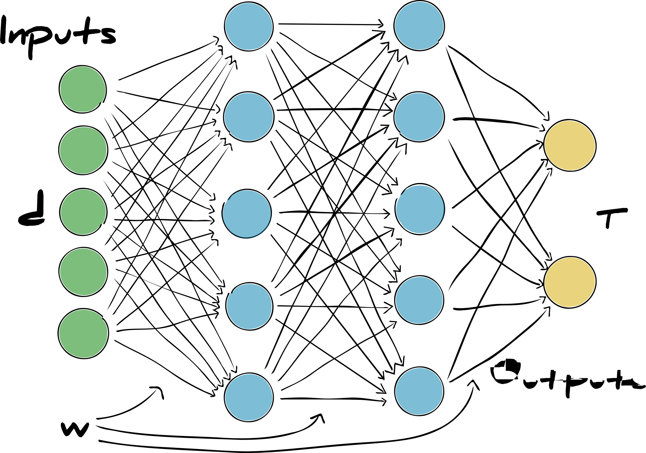
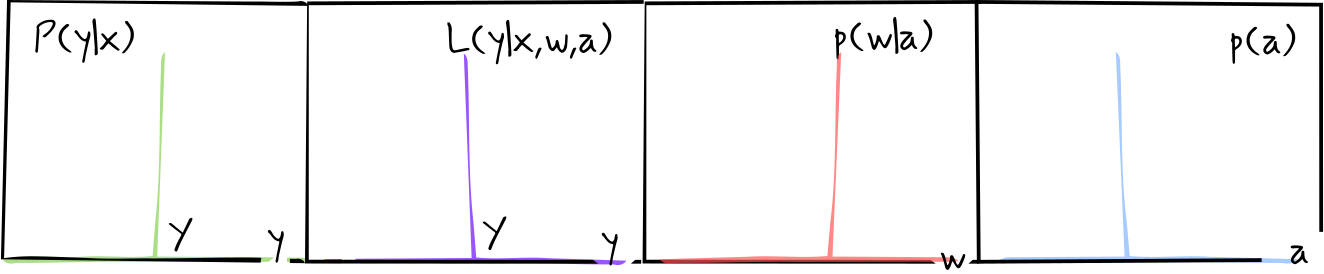
How likely are we to obtain
any particular output from the network
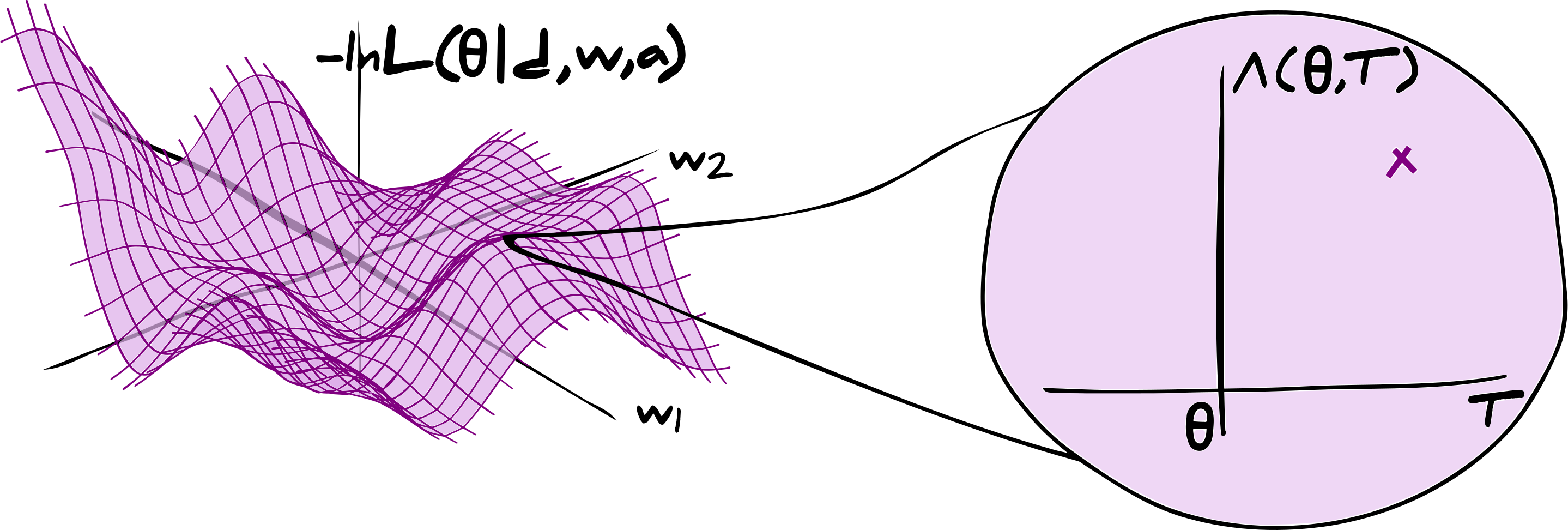
$$\Lambda(\boldsymbol{\theta},\boldsymbol{\tau})\propto-\ln\mathcal{L}(\boldsymbol{\theta}|{\bf d},\boldsymbol{\omega},\boldsymbol{\alpha})$$
The posterior becomes the posterior predictive density
$$\mathcal{P}(\boldsymbol{\theta}|{\bf d}) = \int d\boldsymbol{\omega}d\boldsymbol{\alpha}~\mathcal{L}(\boldsymbol{\theta}|{\bf d},\boldsymbol{\omega},\boldsymbol{\alpha})\mathcal{P}(\boldsymbol{\omega},\boldsymbol{\alpha})$$How likely are the true parameters given some data?
How likely are the parameters to be generated by a particular network?
What is the probability of obtaining a particular network with particular parameter values?
The chance of getting any parameter value from any network given some data is almost equal
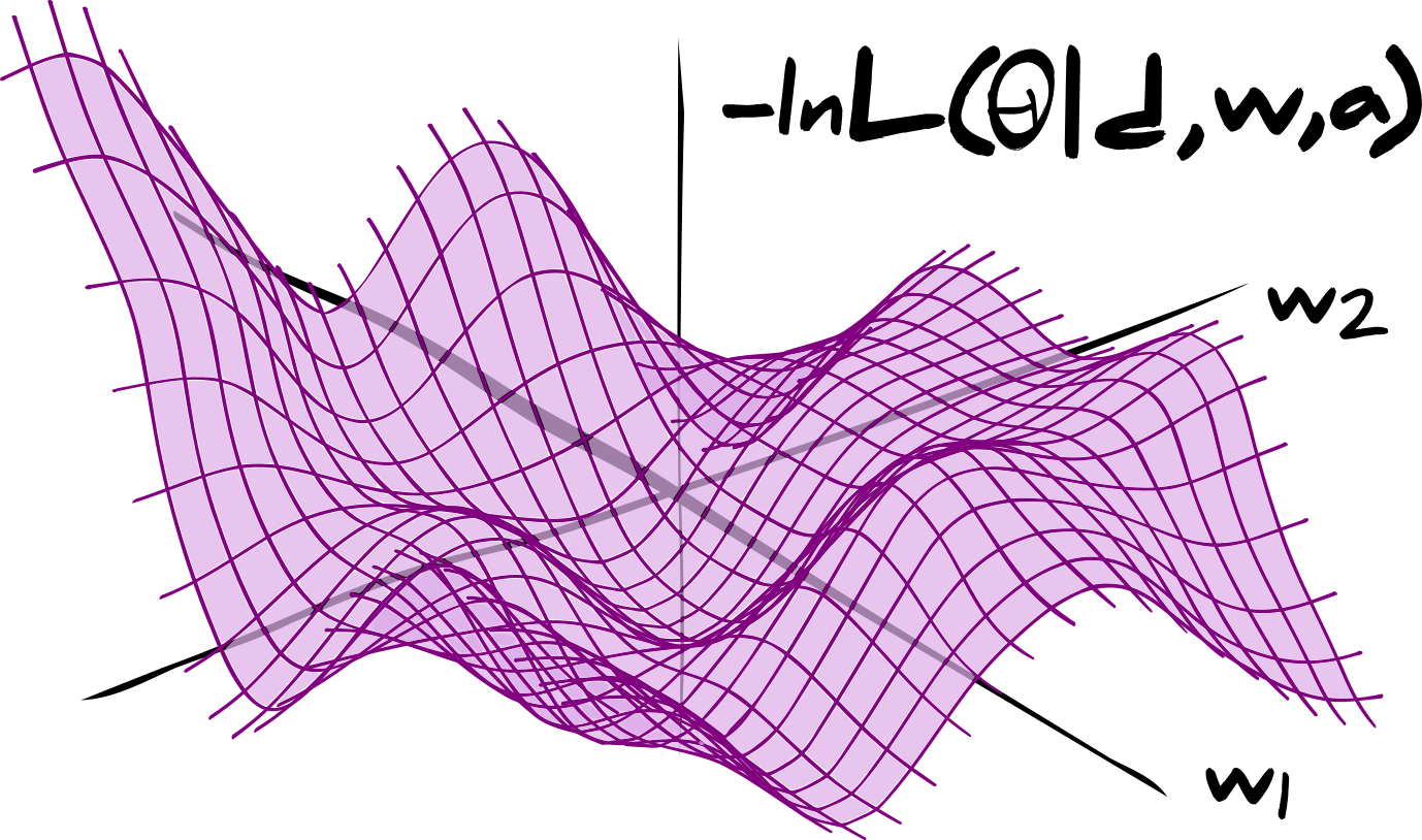
So all the information comes from prior knowledge of the weights and hyperparameters
$$\mathcal{P}(\boldsymbol{\theta}|{\bf d})= \int d\boldsymbol{\omega}d\boldsymbol{\alpha}~\mathcal{L}(\boldsymbol{\theta}|{\bf d},\boldsymbol{\omega},\boldsymbol{\alpha})\mathcal{P}(\boldsymbol{\omega},\boldsymbol{\alpha})$$
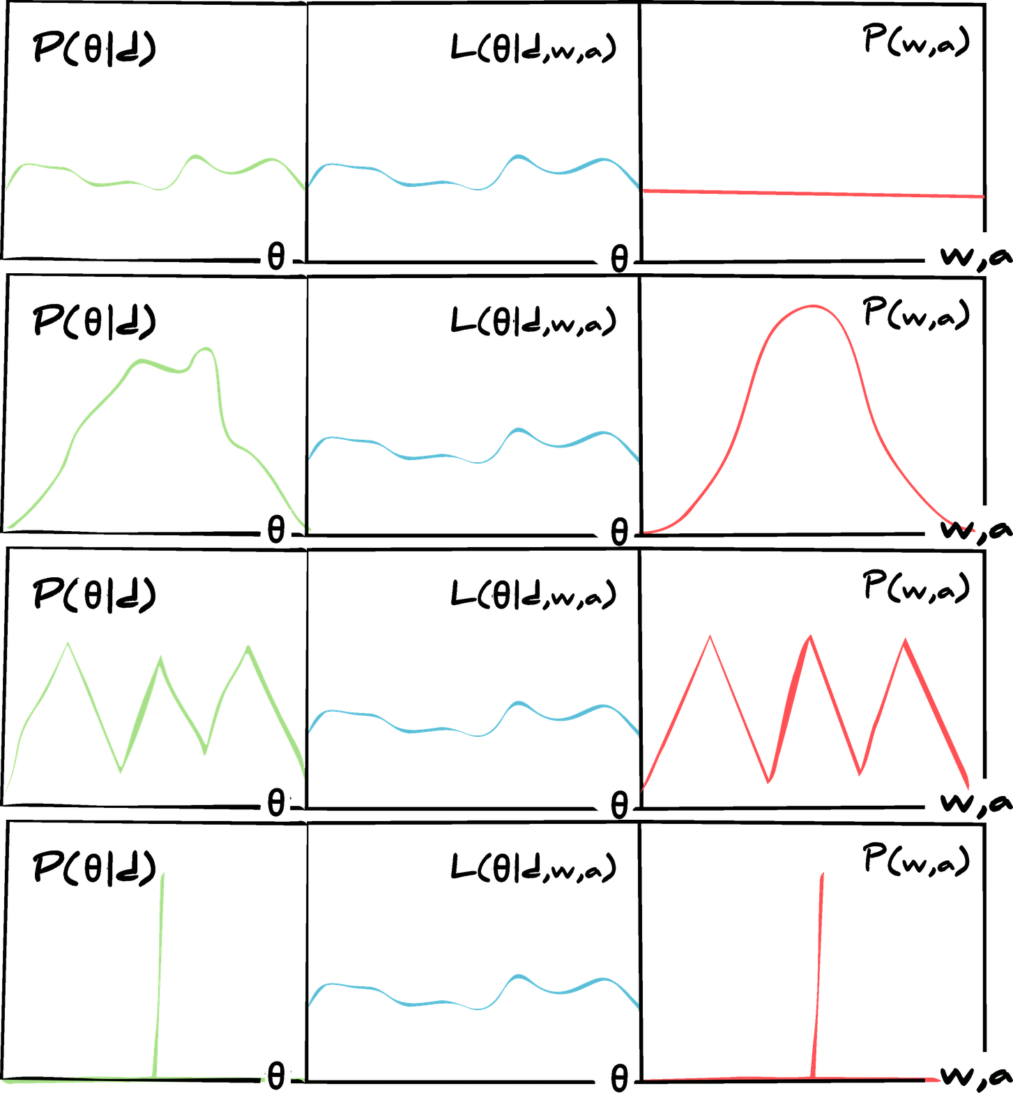
Where does the information about the weights and hyperparameters come from?
Training and validation data
The prior distribution of weights and hyperparameters
becomes the posterior
$$\begin{align*}
&\small\mathcal{P}(\boldsymbol{\omega},\boldsymbol{\alpha}|\boldsymbol{\{}{\bf d},\boldsymbol{\theta}\boldsymbol{\}}^\textrm{train},\boldsymbol{\{}{\bf d},\boldsymbol{\theta}\boldsymbol{\}}^\textrm{val})\propto\\
&\small\phantom{hello}\mathcal{L}(\boldsymbol{\omega},\boldsymbol{\alpha}|\boldsymbol{\{}{\bf d},\boldsymbol{\theta}\boldsymbol{\}}^\textrm{train},\boldsymbol{\{}{\bf d},\boldsymbol{\theta}\boldsymbol{\}}^\textrm{val})p(\boldsymbol{\omega},\boldsymbol{\alpha})
\end{align*}$$
Training a network
What are the maximum likelihood estimates of the weights?
We degenerate the posterior
$$\begin{align*}
\tiny\mathcal{P}(\boldsymbol{\omega},\boldsymbol{\alpha}|\boldsymbol{\{}{\bf d},\boldsymbol{\theta}\boldsymbol{\}}^\textrm{train})\propto&\tiny~\mathcal{L}(\boldsymbol{\omega},\boldsymbol{\alpha}|\boldsymbol{\{}{\bf d},\boldsymbol{\theta}\boldsymbol{\}}^\textrm{train})p(\boldsymbol{\omega},\boldsymbol{\alpha})\\
\tiny\to&\tiny~\delta(\boldsymbol{\omega}-\boldsymbol{\omega}^\textrm{MLE},\boldsymbol{\alpha}-\boldsymbol{\alpha}^*)
\tiny\\
\tiny\mathcal{P}(\boldsymbol{\theta}|{\bf d}) \propto&\tiny~\int d\boldsymbol{\omega}d\boldsymbol{\alpha}\mathcal{L}(\boldsymbol{\theta}|{\bf d},\boldsymbol{\omega},\boldsymbol{\alpha})\delta(\boldsymbol{\omega}-\boldsymbol{\omega}^\textrm{MLE},\boldsymbol{\alpha}-\boldsymbol{\alpha}^*)\\
\tiny=&\tiny~\delta(\boldsymbol{\tau})
\end{align*}$$
All predictions are (unknowably incorrect) estimates
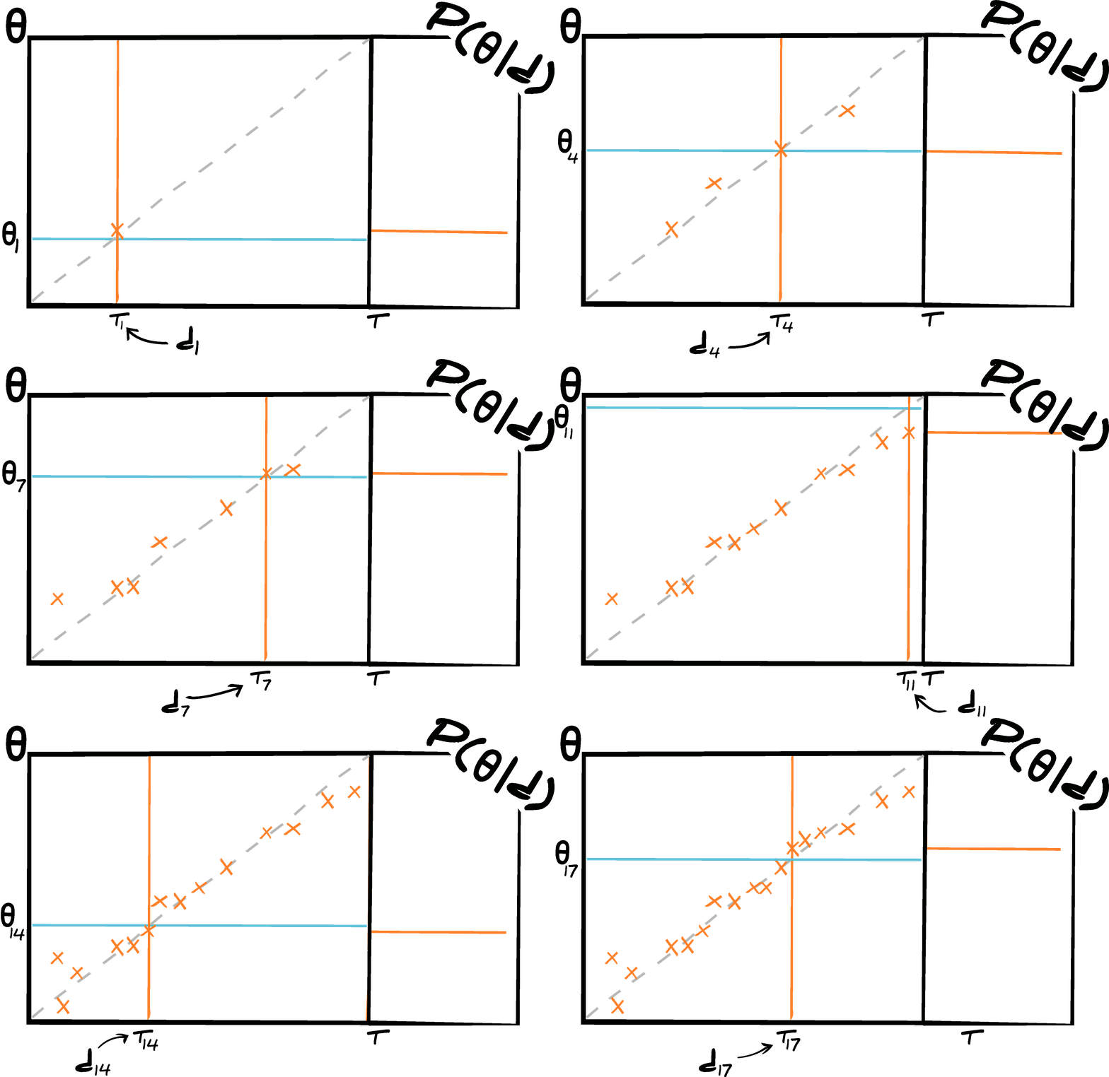
$$\mathcal{P}(\boldsymbol{\theta}|{\bf d})=\delta(\boldsymbol{\tau})$$
There is no way to interpret how close $\boldsymbol{\tau}$ is to $\boldsymbol{\theta}$...
Local maximum likelihood estimates
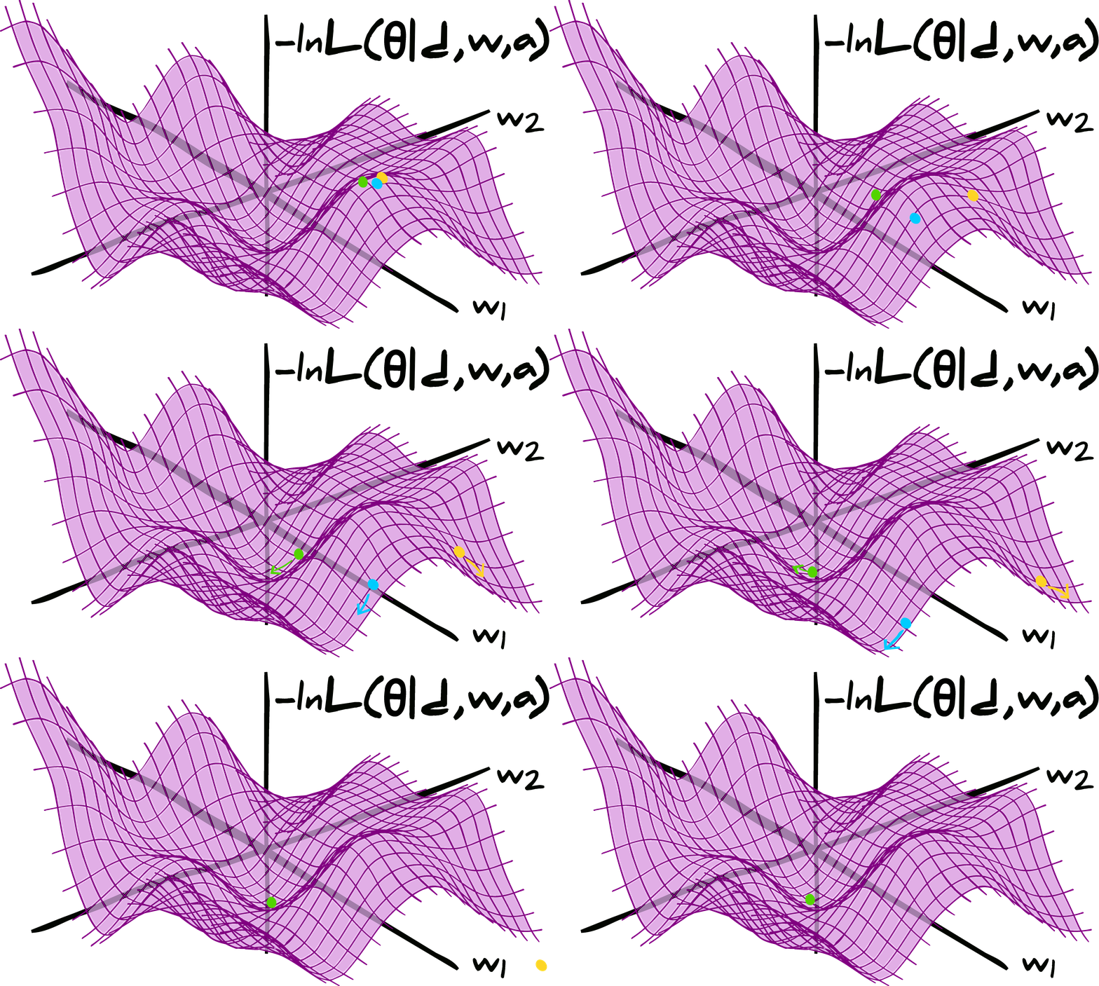
Are there better methods?
Variational inference
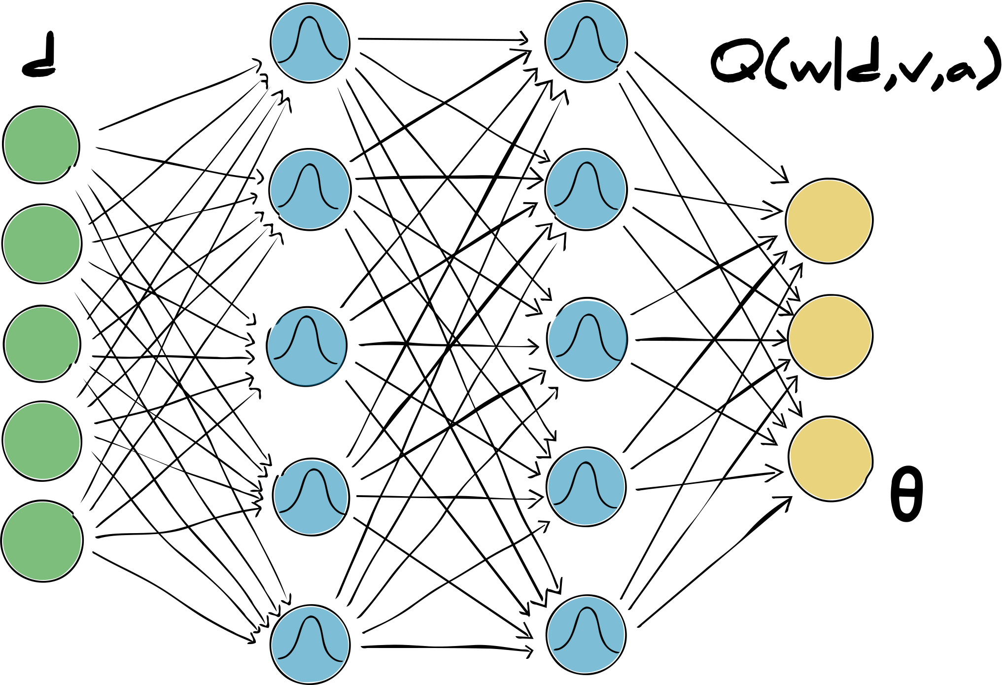
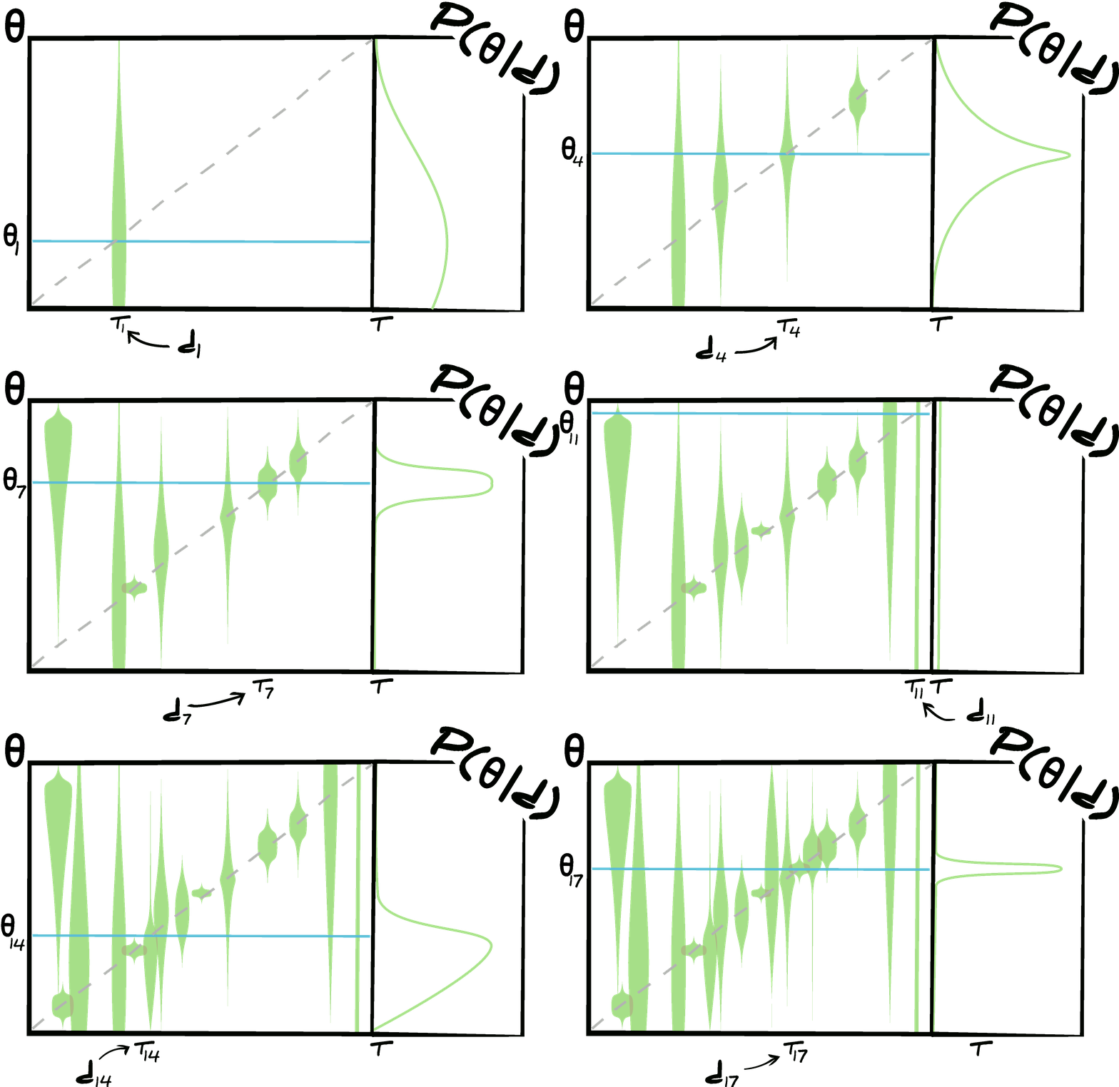
Still depends on fixed weights in the complex likelihood surface
and choice of variational distribution
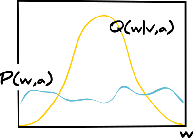 $$\begin{align*}
\mathcal{P}(\boldsymbol{\theta}|{\bf d})&=\int d\boldsymbol{\omega}d\boldsymbol{\nu}d\boldsymbol{\alpha}~\mathcal{L}(\boldsymbol{\theta}|{\bf d},\boldsymbol{\omega},\boldsymbol{\alpha})\mathcal{Q}(\boldsymbol{\omega}|\boldsymbol{\nu}, \boldsymbol{\alpha}, \boldsymbol{\{}{\bf d}, \boldsymbol{\theta}\boldsymbol{\}}^\textrm{train})\\
&\phantom{hellohello}\times\delta(\boldsymbol{\nu}-\boldsymbol{\nu}^\textrm{MLE}, \boldsymbol{\alpha}-\boldsymbol{\alpha}^*)\\
&=\int d\boldsymbol{\omega}~\mathcal{L}(\boldsymbol{\theta}|{\bf d},\boldsymbol{\omega}, \boldsymbol{\alpha}^*)\mathcal{Q}(\boldsymbol{\omega}|\boldsymbol{\nu}^\textrm{MLE}, \boldsymbol{\alpha}^*, \boldsymbol{\{}{\bf d}, \boldsymbol{\theta}\boldsymbol{\}}^\textrm{train}).
\end{align*}$$
$$\begin{align*}
\mathcal{P}(\boldsymbol{\theta}|{\bf d})&=\int d\boldsymbol{\omega}d\boldsymbol{\nu}d\boldsymbol{\alpha}~\mathcal{L}(\boldsymbol{\theta}|{\bf d},\boldsymbol{\omega},\boldsymbol{\alpha})\mathcal{Q}(\boldsymbol{\omega}|\boldsymbol{\nu}, \boldsymbol{\alpha}, \boldsymbol{\{}{\bf d}, \boldsymbol{\theta}\boldsymbol{\}}^\textrm{train})\\
&\phantom{hellohello}\times\delta(\boldsymbol{\nu}-\boldsymbol{\nu}^\textrm{MLE}, \boldsymbol{\alpha}-\boldsymbol{\alpha}^*)\\
&=\int d\boldsymbol{\omega}~\mathcal{L}(\boldsymbol{\theta}|{\bf d},\boldsymbol{\omega}, \boldsymbol{\alpha}^*)\mathcal{Q}(\boldsymbol{\omega}|\boldsymbol{\nu}^\textrm{MLE}, \boldsymbol{\alpha}^*, \boldsymbol{\{}{\bf d}, \boldsymbol{\theta}\boldsymbol{\}}^\textrm{train}).
\end{align*}$$
Bayesian neural networks
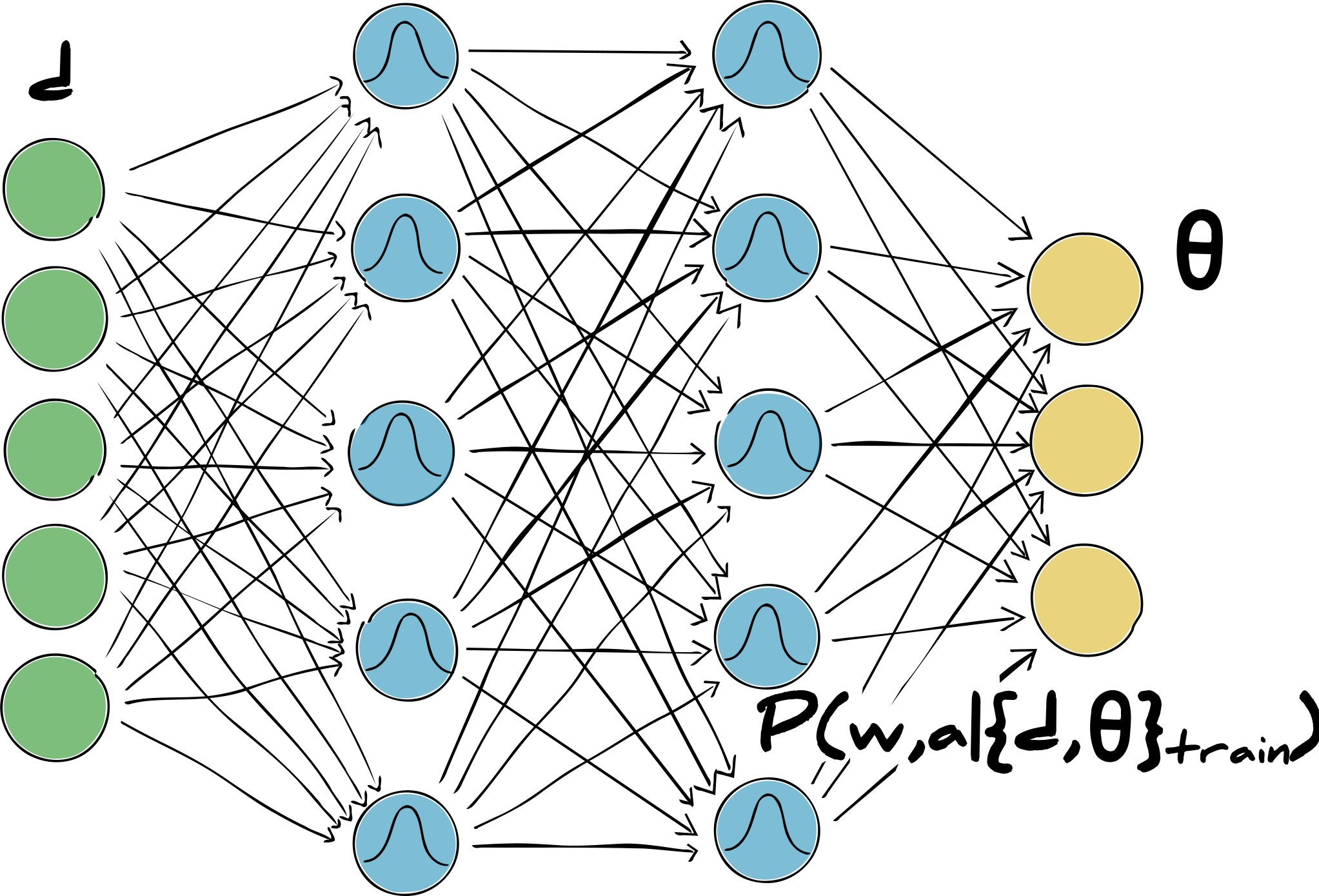
Approximate the posterior distribution of weights and hypermeters
$$\begin{align*} \small\mathcal{P}(\boldsymbol{\theta}|{\bf d}) =&\small~\int d\boldsymbol{\omega}d\boldsymbol{\alpha}~\mathcal{L}(\boldsymbol{\theta}|{\bf d}, \boldsymbol{\omega}, \boldsymbol{\alpha})\mathcal{P}(\boldsymbol{\omega},\boldsymbol{\alpha}|\boldsymbol{\{}{\bf d}, \boldsymbol{\theta}\boldsymbol{\}}^\textrm{train})\\ \propto&~\int d\boldsymbol{\omega}d\boldsymbol{\alpha}~\mathcal{L}(\boldsymbol{\theta}|{\bf d}, \boldsymbol{\omega}, \boldsymbol{\alpha})\\ &\phantom{hello}\times \prod_i^{n_\textrm{train}}\mathcal{L}(\boldsymbol{\theta}^\textrm{train}_i|{\bf d}_i^\textrm{train}, \boldsymbol{\omega},\boldsymbol{\alpha})p(\boldsymbol{\omega},\boldsymbol{\alpha}).\phantom{hello} \end{align*} $$Everything is dependent on the training data!
Classical network : $\tiny \mathcal{P}(\boldsymbol{\omega},\boldsymbol{\alpha}|\boldsymbol{\{}{\bf d},\boldsymbol{\theta}\boldsymbol{\}}^\textrm{train}) \to \delta(\boldsymbol{\omega}-\boldsymbol{\omega}^\textrm{MLE},\boldsymbol{\alpha}-\boldsymbol{\alpha}^*)$
Variational inference : $\tiny \mathcal{P}(\boldsymbol{\omega},\boldsymbol{\alpha}|\boldsymbol{\{}{\bf d},\boldsymbol{\theta}\boldsymbol{\}}^\textrm{train}) = \mathcal{Q}(\boldsymbol{\omega}|\boldsymbol{\nu}^\textrm{MLE}, \boldsymbol{\alpha}^*, \boldsymbol{\{}{\bf d},\boldsymbol{\theta}\boldsymbol{\}}^\textrm{train})$
Bayesian networks : $\tiny \mathcal{P}(\boldsymbol{\omega},\boldsymbol{\alpha}|\boldsymbol{\{}{\bf d},\boldsymbol{\theta}\boldsymbol{\}}^\textrm{train}) =\prod_i^{n_\textrm{train}}\mathcal{L}({\bf t}^\textrm{train}_i|\boldsymbol{\theta}^\textrm{train}_i,\boldsymbol{\omega},\boldsymbol{\alpha})p(\boldsymbol{\omega},\boldsymbol{\alpha})$
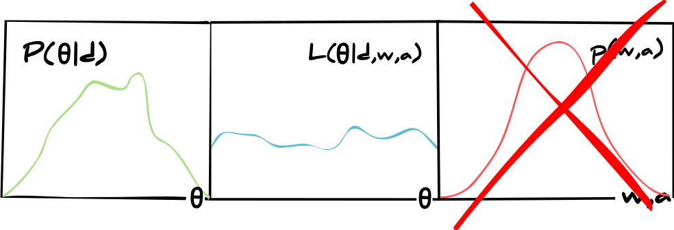
If the training data, network optimisation, or (pretty much) anything else is not perfect, the inference will be biased
Parameter inference with summaries
Consider when the likelihood of some data, $\mathcal{L}({\bf d}|\boldsymbol{\theta})$ is unknown
Summarise the data, $\mathscr{f}:{\bf d}\to{\bf t}$, to have a nicer likelihood for the model $\mathcal{M}\otimes\mathscr{f}:\boldsymbol{\theta}\to{\bf t}$
$$
\mathcal{P}(\boldsymbol{\theta}|{\bf t},\mathcal{M}\otimes\mathscr{f}) = \frac{\mathcal{L}({\bf t}|\boldsymbol{\theta},\mathcal{M}\otimes\mathscr{f})p(\boldsymbol{\theta}|\mathcal{M})}{p({\bf t}|\mathcal{M}\otimes\mathscr{f})}
$$
The data no longer enters the inference, only the summaries
We can use a neural network as this summarising function
But the likelihood of the summaries is still difficult in this situtation
Forward modelling
Method 1 :
Likelihood-free inference
Use the same neural network to summarise observations and simulations
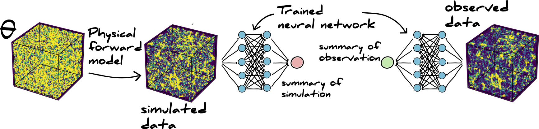
Generate simulations drawn from prior and summarise
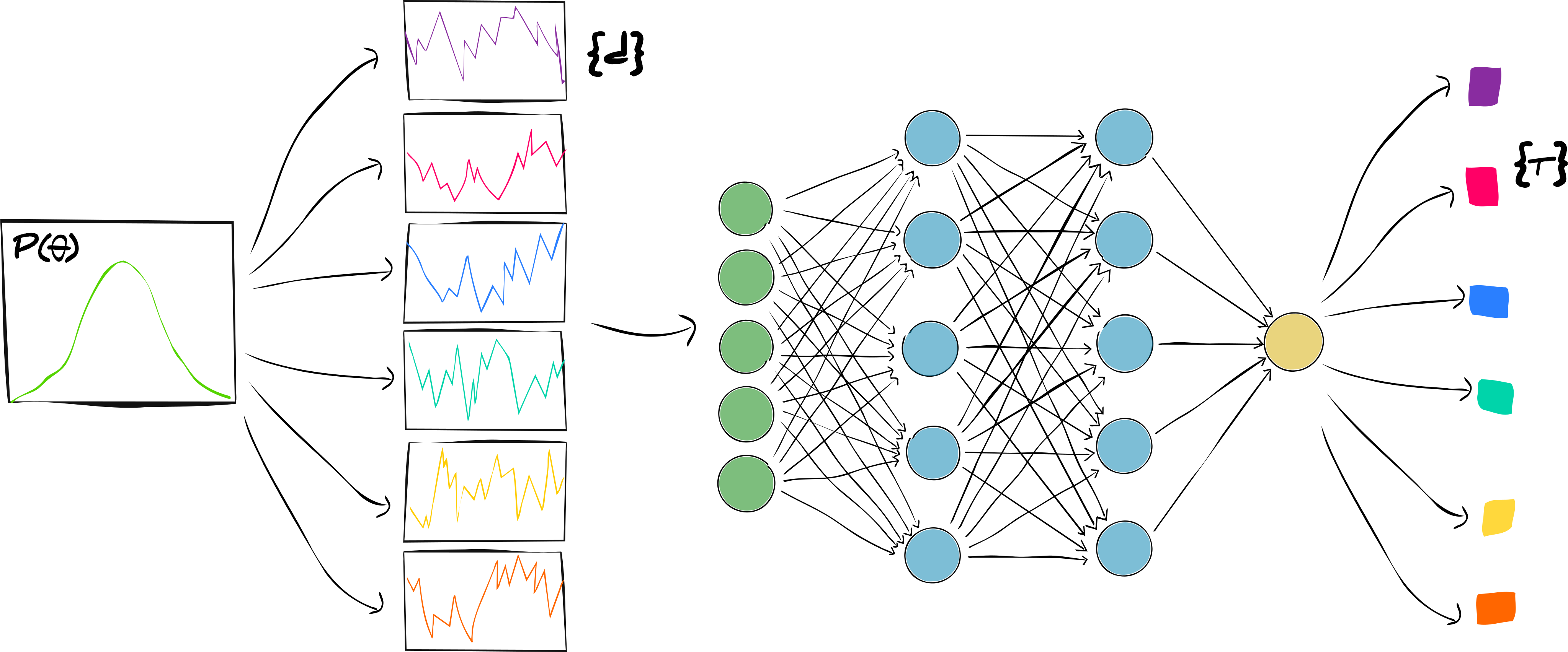
Make a kernel density estimate (or use ABC) on the simulations
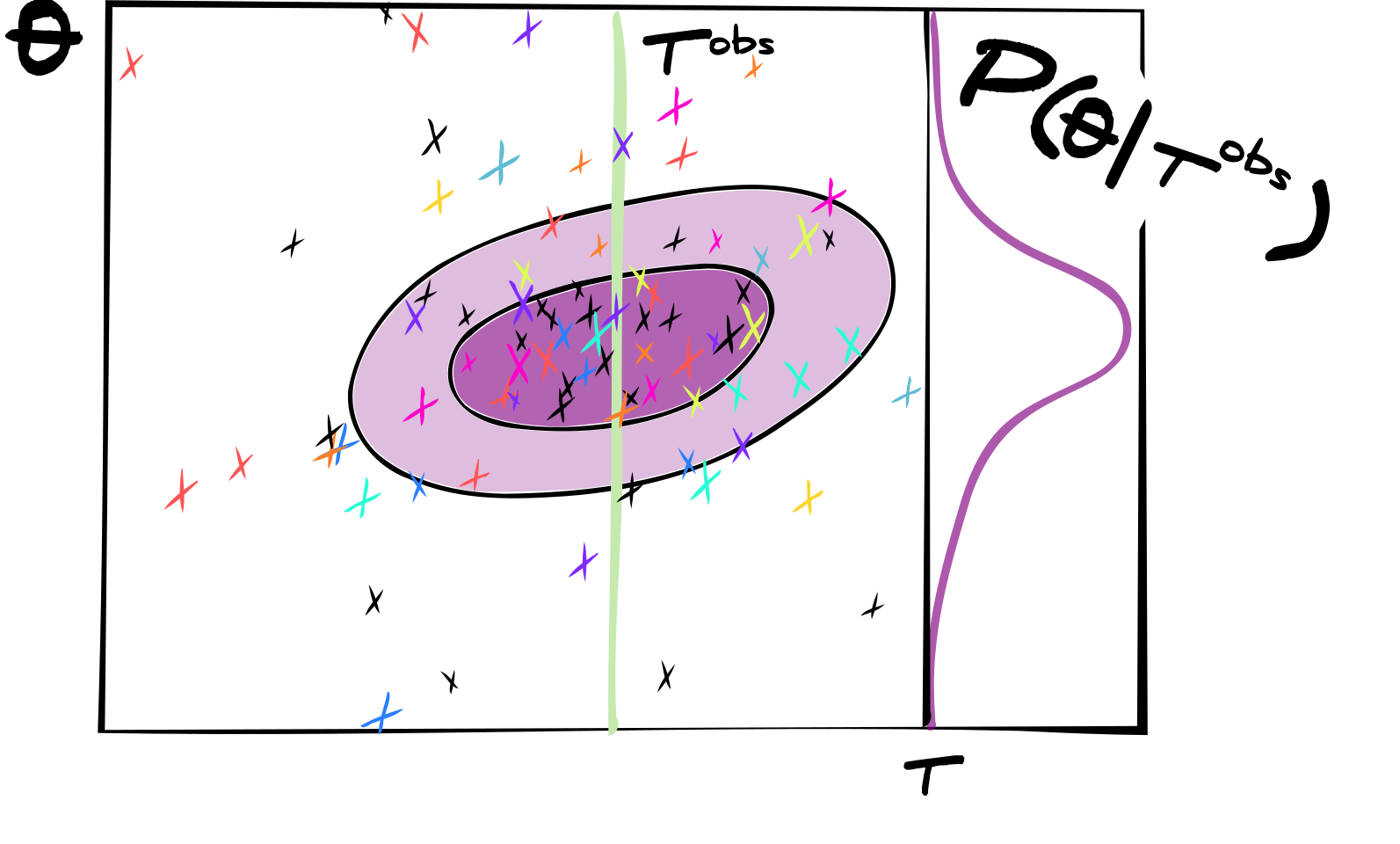 A slice through at the summarised observation is the approximate posterior
Posterior distribution of galaxy counts and fluxes in fields
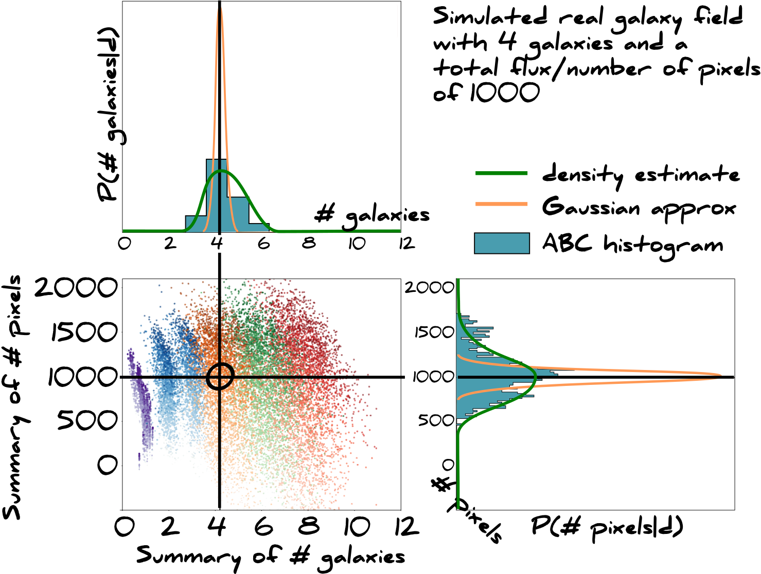
We're still biased by the form of the density estimator we use, and by the number of simulations we use for approximating the posterior
Method 2 :
Infer the data, physics and neural network
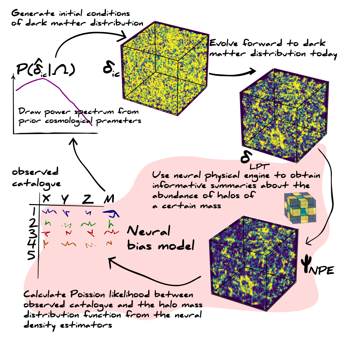
Use neural physical engines