For a bit of early morning compression fun why not run¶

pip install IMNN jupyter matplotlib
git clone https://github.com/tomcharnock/IMNN-LFI_Taskforce.git
cd IMNN-LFI_Taskforce
jupyter notebook

or go to

tinyurl.com/LFI-IMNN

Information maximising neural networks for dimensionality reduction¶

Tom Charnock

Institut d'Astrophysique de Paris

Notebook: presentations.charnock.fr/IMNN/LFI_Taskforce

pip install IMNN jupyter matplotlib
git clone https://github.com/tomcharnock/IMNN-LFI_Taskforce.git
cd IMNN-LFI_Taskforce
jupyter notebook

tinyurl.com/LFI-IMNN

Dimensionality reduction¶

Data is big!¶

Euclid-like survey

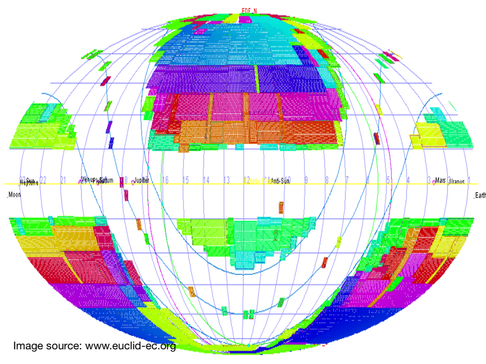
(~10$^\textsf{4}$TB data, ~10$^\textsf{5}$ images, ~10$^\textsf{9}$ sources, ~10$^\textsf{6}$ redshifts)

Even the number of summary statistics is $\sim$10$^\textsf{4}$!¶

Some (slightly) smaller simpler data¶

Gaussian data with $n_{\bf d}=10$ and variance $\Sigma = 1$

In [25]:

real_data = simulator(np.array([[1.]]),
                      np.random.randint(int(1e6)),
                      {"input shape": [10]})
plot_real_data(real_data)

Why do we need data reduction?¶

Approximate Bayesian computation¶

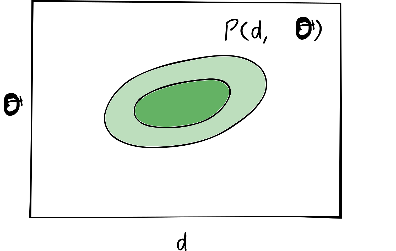
For LFI (and in particular ABC) we work in the space of data ${\bf d}$ and model parameters $\boldsymbol{\theta}$

Posterior is a slice through this space at some given data

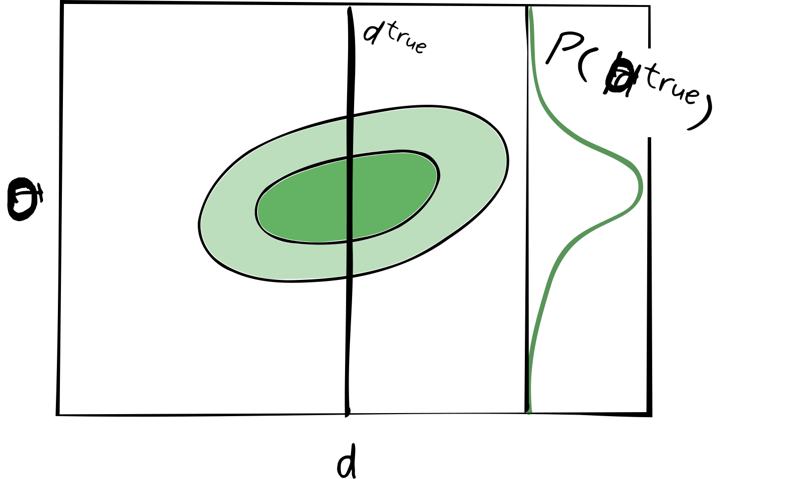
ABC posterior¶

Simulate the data and accept simulations close to the true data

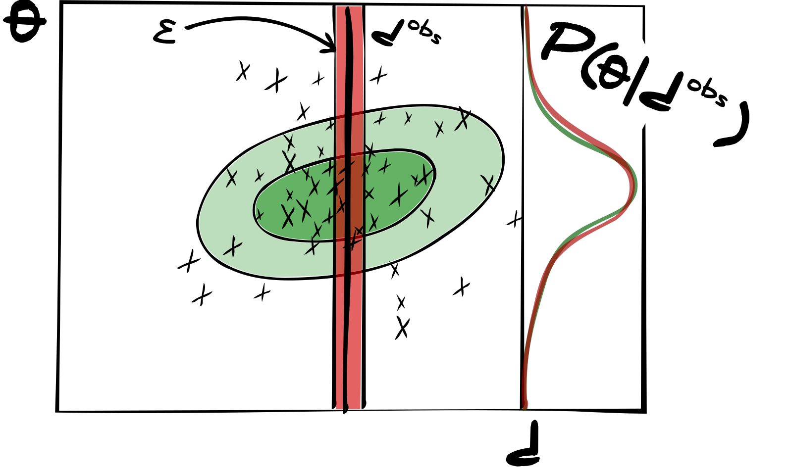
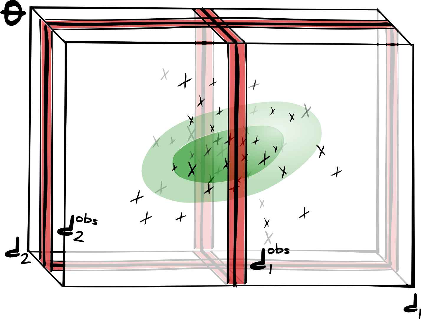
The curse of dimensionality¶

The higher the dimension of the data, the less likely any simulation will actually look like the true data

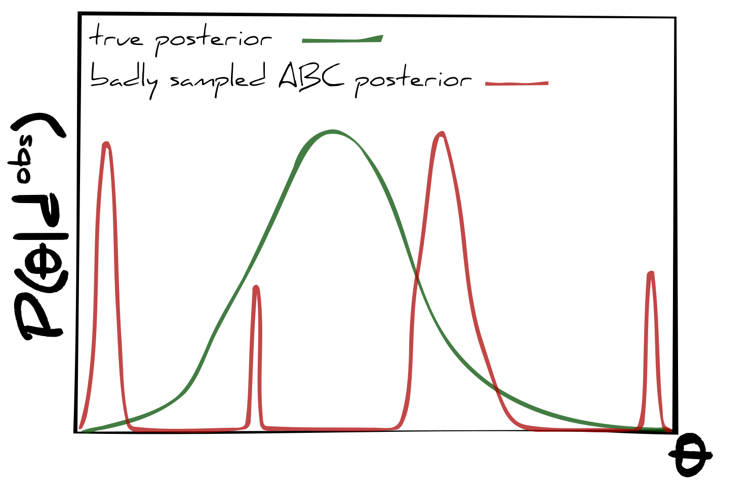
Inadequate sampling¶

Impossibly large numbers of simulations become necessary to correctly sample the posterior

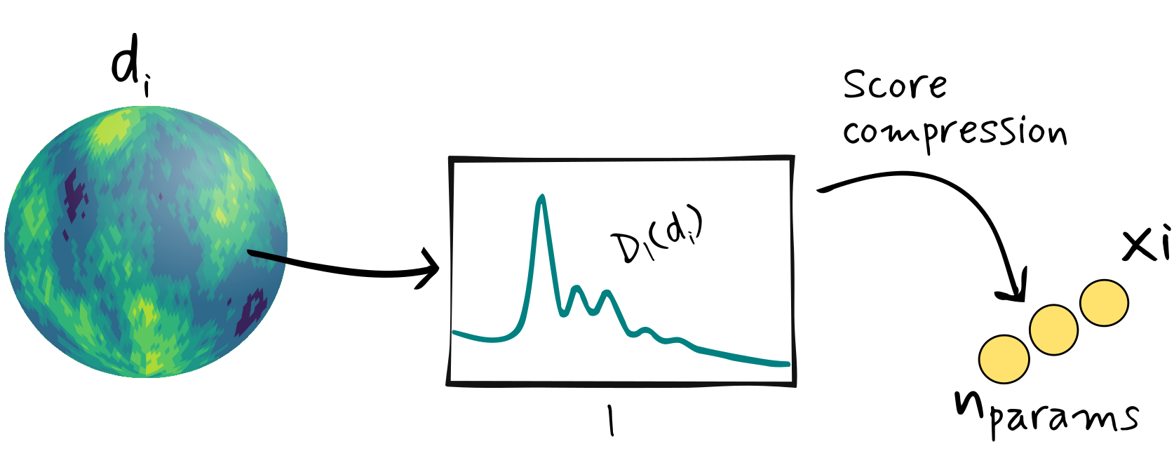
Methods for dimensionality reduction¶

Informative compressed summaries¶

The information inequality provides a natural description of

optimal compressed summaries¶

We define optimal statistics as the set of summaries which saturate the information inequality

$$Cov\left[{\bf x}_\alpha,{\bf x}_\beta\right] \ge \frac{\partial\langle{\bf x}_\mu\rangle}{\partial\theta_\alpha} {\bf F}^{-1}_{\mu\nu}\frac{\partial\langle{\bf x}_\nu\rangle}{\partial\theta_\beta}$$

Fisher information¶

Amount of information some data, ${\bf d}$, contains about model parameters, $\boldsymbol{\theta}$, with likelihood $\mathcal{L}({\bf d}|\boldsymbol{\theta})$

$$\begin{align*} {\bf F}_{\alpha\beta} & = - \left.\left\langle\frac{\partial^2\ln\mathcal{L}({\bf d}|\boldsymbol{\theta})}{\partial\theta_\alpha\partial\theta_\beta}\right\rangle\right|_{\boldsymbol{\theta}^\textrm{fid}}\\ & = \phantom{-}\left.\left\langle\frac{\partial\ln\mathcal{L}({\bf d}|\boldsymbol{\theta})}{\partial\theta_\alpha}\frac{\partial\ln\mathcal{L}({\bf d}|\boldsymbol{\theta})}{\partial\theta_\beta}\right\rangle\right|_{\boldsymbol{\theta}^\textrm{fid}} \end{align*}$$

Expectation of the square of the score function at some fiducial model parameter values¶

How to build optimal compressed summaries¶

Start by expanding a generalised log-likelihood about some fiducial parameters, $\boldsymbol{\theta}^\textsf{fid}$ $$\begin{align*} \ln\mathcal{L}({\bf d}|\boldsymbol{\theta})\phantom{+} =&\phantom{+} \ln\mathcal{L}({\bf d}|\boldsymbol{\theta}^\textrm{fid})+\delta\theta_\alpha^T\frac{\partial\ln\mathcal{L}({\bf d}|\boldsymbol{\theta}^\textrm{fid})}{\partial\theta_\alpha}\\ &\phantom{+}+\frac{1}{2}\delta\theta_\alpha^T\frac{\partial^2\ln\mathcal{L}({\bf d}|\boldsymbol{\theta}^\textrm{fid})}{\partial\theta_\alpha\partial\theta_\beta}\delta\theta_\beta + \cdots \end{align*}$$

To linear order, the data only couples to the log-likelihood through the score fuction at some fiducial parameters

Use the score function as a set of summaries¶

$${\bf x}_\alpha = \frac{\partial\ln\mathcal{L}({\bf d}|\boldsymbol{\theta}^\textrm{fid})} {\partial\theta_\alpha}$$

This is a set of sufficient* statistics which saturate the information inequality

$$Cov\left[{\bf x}_\alpha,{\bf x}_\beta\right] = \frac{\partial\langle{\bf x}_\mu\rangle}{\partial\theta_\alpha}{\bf F}^{-1}_{\mu\nu}\frac{\partial\langle{\bf x}_\nu\rangle}{\partial\theta_\beta}$$

Since gradient of the expectation value of the summaries (evaluated at the fiducial parameter values) is

$$\begin{align*} \frac{\partial\langle{\bf x}_\beta\rangle}{\partial\theta_\alpha}= & \phantom{=}\left.\left\langle\frac{\partial^2\ln\mathcal{L}({\bf d}|\boldsymbol{\theta})}{\partial\theta_\alpha\partial\theta_\beta}\right\rangle\right|_{\boldsymbol{\theta}^\textrm{fid}}\\ = & \phantom{=}-{\bf F}_{\alpha\beta} \end{align*}$$

such that

$$\frac{\partial\langle{\bf x}_\mu\rangle}{\partial\theta_\alpha}{\bf F}^{-1}_{\mu\nu}\frac{\partial\langle{\bf x}_\nu\rangle}{\partial\theta_\beta} = {\bf F}_{\alpha\beta}$$

and the covariance of the summaries is

$$\begin{align*} Cov\left[{\bf x}_\alpha, {\bf x}_\beta\right] = & \left.\left\langle\frac{\partial\ln\mathcal{L}({\bf d}|\boldsymbol{\theta})}{\partial\theta_\alpha}\frac{\partial\ln\mathcal{L}({\bf d}|\boldsymbol{\theta})}{\partial\theta_\beta}\right\rangle\right|_{\boldsymbol{\theta}^\textrm{fid}}\\ =& {\bf F}_{\alpha\beta} \end{align*}$$

then ${\bf x}_\alpha$ saturate the information inequality

$$Cov\left[{\bf x}_\alpha,{\bf x}_\beta\right] = \frac{\partial\langle{\bf x}_\mu\rangle}{\partial\theta_\alpha}{\bf F}^{-1}_{\mu\nu}\frac{\partial\langle{\bf x}_\nu\rangle}{\partial\theta_\beta}$$

The score function defines optimal compressed summaries¶

Informative compressed summaries¶

MASSIVE dimensionality compression

$$\mathbb{R}^{n_{\bf d}}\to\mathbb{R}^{n_\textrm{params}}$$

$$\hat{\boldsymbol{\theta}}_\alpha = \boldsymbol{\theta}^\textrm{fid}_\alpha + {\bf F}^{-1}_{\alpha\beta}{\bf x}_\beta$$

We just need to know how to take the partial derivative of the log-likelihood

$${\bf x}_\alpha = \frac{\partial\ln\mathcal{L}({\bf d}|\boldsymbol{\theta}^\textrm{fid})}{\partial\theta_\alpha}$$

Great... but we're at a LIKELIHOOD-FREE inference workshop¶

We can try and approximate the likelihood¶

If the likelihood of our data is Gaussian:

this problem is solved with lossless summaries
this is MOPED compression

If our likelihood is known to linear order:

this problem is solved with lossless summaries

If the likelihood of our data is nearly-Gaussian:

this problem is basically solved with not-quite-lossless summaries

If our data has known useful summaries
(for example the power spectrum):

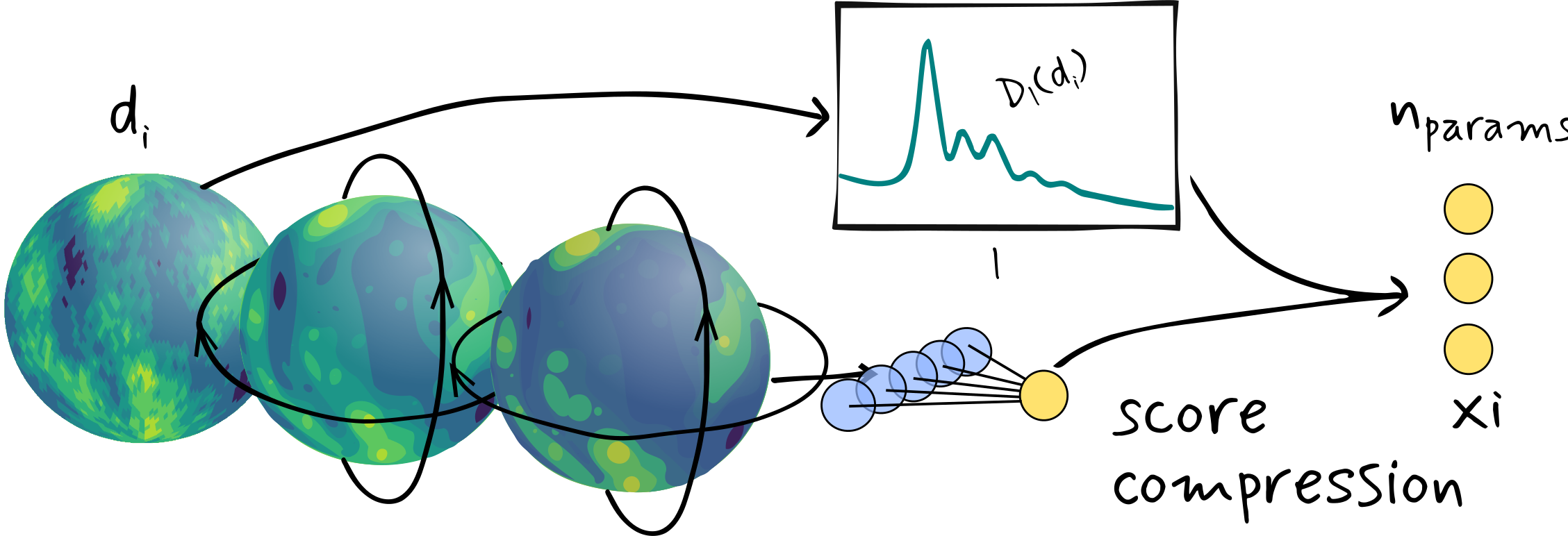
we can compress the data to the useful summaries
then compress the summaries using score compression

Can we be more general than this though?¶

Yes!¶

Information maximising neural networks¶

Load the (very easy to use) module¶

pip install IMNN

or github.com/tomcharnock/IMNN

In [26]:

from IMNN import IMNN

Non-linear compression function¶

So how do we find this magic function?¶

Find the function which gives Gaussian summaries¶

We find a way to map the data to some summaries $\mathscr{f}:{\bf d}\to{\bf x}$, where ${\bf x}$ are described by

$$-2\ln\mathcal{L}({\bf x}|\boldsymbol{\theta}) = ({\bf x}-\mu_\mathscr{f}(\boldsymbol{\theta}))^T{\bf C}^{-1}_\mathscr{f}({\bf x}-\mu_\mathscr{f}(\boldsymbol{\theta}))$$

where $\mu_\mathscr{f}(\boldsymbol{\theta})$ and ${\bf C}_\mathscr{f}$ are the mean and covariance an ensemble of summaries mapped from fiducial simulations.

This function is a trained neural network¶

optimised to maximise the Fisher information!¶

$$\textsf{Loss} = -\ln\det{\bf F}_{\alpha\beta} + \lambda||{\bf C}_\mathscr{f}-\mathbb{I}||_2$$

Fisher information given our known Gaussian likelihood of summaries¶

$${\bf F}_{\alpha\beta} = \frac{\partial\mu_\mathscr{f}}{\partial\theta_\alpha}^T{\bf C}_\mathscr{f}^{-1}\frac{\partial\mu_\mathscr{f}}{\partial\theta_\beta}$$

Unbiased parameter estimate straight from the IMNN¶

$$\hat{\boldsymbol{\theta}}_\alpha = \boldsymbol{\theta}^\textrm{fid}_\alpha + {\bf F}^{-1}_{\alpha\beta}{\bf C}_\mathscr{f}^{-1}\frac{\partial\mu_\mathscr{f}}{\partial\theta_\beta}({\bf x} - \mu_\mathscr{f})$$

Training the network¶

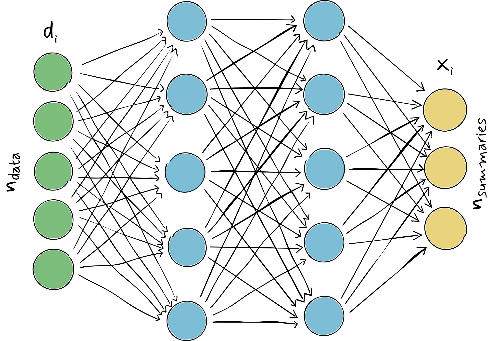
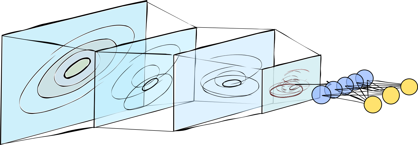
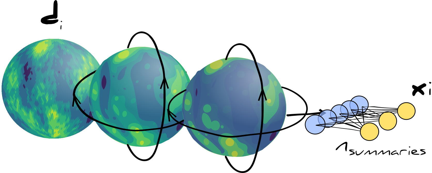
Build the network to best exploit the data¶

Fully connected networks when you don't know better
(oddly distributed data)

Convolutions for translationally invariant data
(images or local signals)

Other specialised architectures
(spherical convolutional networks for cosmological maps)

We can build the network to work on summaries with unknown likelihoods¶

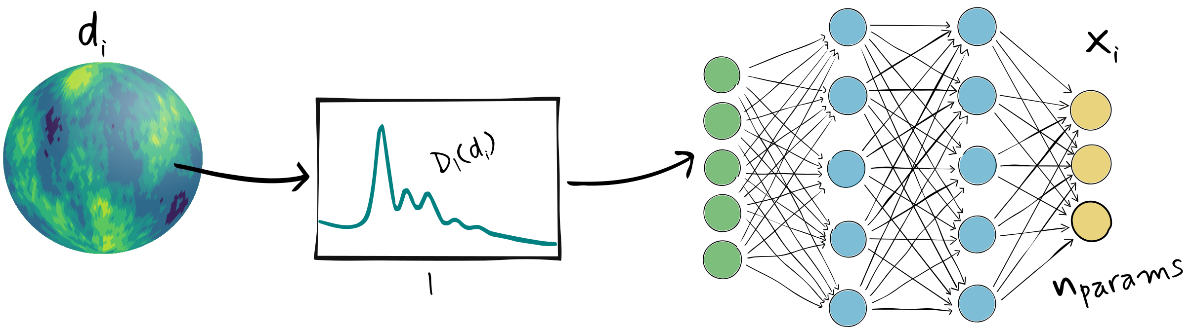
Finding that one extra summary...¶

We can combine the IMNN with our known and loved summaries to extract just that little bit extra information

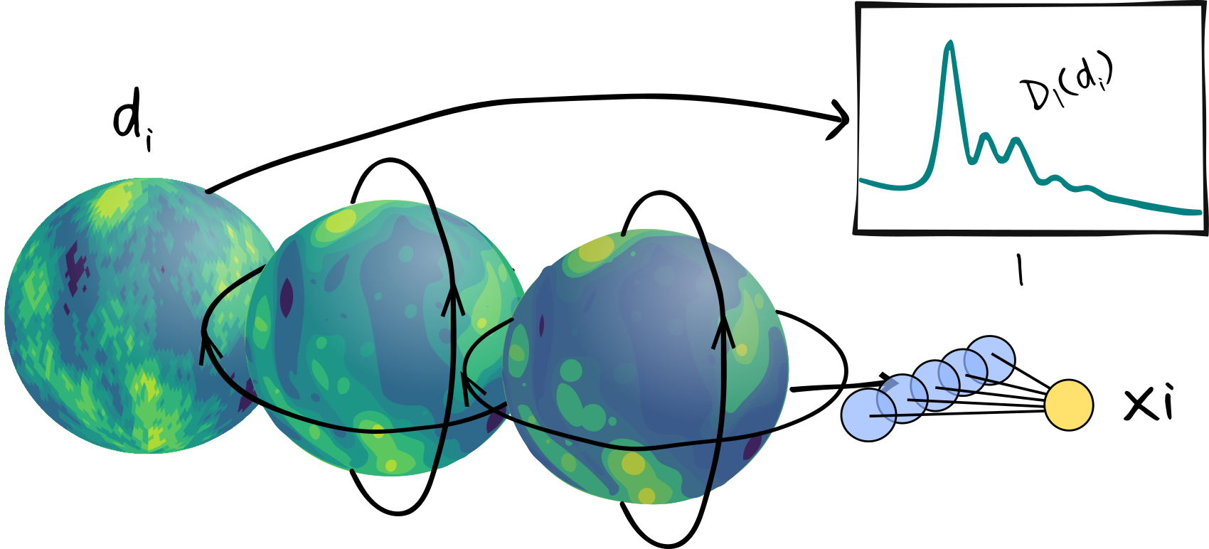
Of course we can still do score compression¶

Define our network¶

In [27]:

def network(input_tensor):
    x = tf.nn.leaky_relu(dense(input_tensor, 128, "layer_1"), 0.01)
    x = tf.nn.leaky_relu(dense(x, 128, "layer_2"), 0.01)
    return dense(x, imnn.n_summaries, "output")

Generate training (and validation) data¶

Massively cheap¶

We only need simulations at the fiducial parameter values!

In [28]:

n_s = 1000
n_p = 100
num_summaries = 1
fiducial = [1.]
h = [0.1]
input_shape = [10]

In [29]:

data = generate_data(n_train, n_s, n_p, input_shape, fiducial, h, np.random.randint(int(1e6)))
plot_data(data)

Let's build the IMNN¶

In [30]:

imnn = IMNN.IMNN(
    {"number of simulations": n_s,
     "number of derivative simulations": n_p,
     "fiducial": fiducial,
     "number of summaries": num_summaries,
     "input shape": input_shape,
     "dtype": 32})

In [31]:

imnn.setup(network = network, load_data = data)

WARNING:tensorflow:From /Users/charnock/.pyenv/versions/3.6.6/lib/python3.6/site-packages/tensorflow/python/framework/op_def_library.py:263: colocate_with (from tensorflow.python.framework.ops) is deprecated and will be removed in a future version.
Instructions for updating:
Colocations handled automatically by placer.
WARNING:tensorflow:From /Users/charnock/.pyenv/versions/3.6.6/lib/python3.6/site-packages/tensorflow/python/ops/math_ops.py:3066: to_int32 (from tensorflow.python.ops.math_ops) is deprecated and will be removed in a future version.
Instructions for updating:
Use tf.cast instead.

Pass $n_\textrm{sims}$ simulations through the network and calculate ${\bf C}_\mathscr{f}$¶

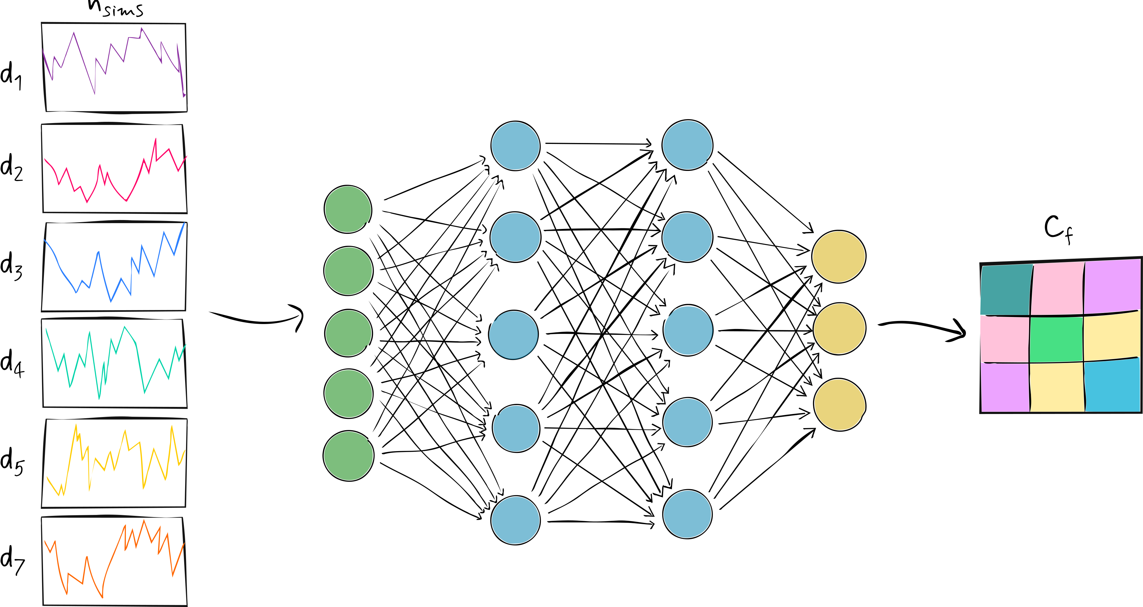
Calculate the derivative of the network outputs with respect to the parameters¶

$$\frac{\partial\mu_\mathscr{f}}{\partial\theta_\alpha} = \frac{1}{n_\textrm{p}}\sum_{i=1}^{n_\textrm{p}}\frac{\partial{\bf x}_i}{\partial{\bf d}_i}\frac{\partial{\bf d}_i}{\partial\theta_\alpha}$$

Calculate the Fisher information¶

$${\bf F}_{\alpha\beta} = \frac{\partial\mu_\mathscr{f}}{\partial\theta_\alpha}^T{\bf C}_\mathscr{f}^{-1}\frac{\partial\mu_\mathscr{f}}{\partial\theta_\beta}$$

Update the network parameters using the gradient of the loss function¶

$$\textsf{Loss} = -\ln\det{\bf F}_{\alpha\beta} + \lambda||{\bf C}_\mathscr{f}-\mathbb{I}||_2$$

Lather, rince, repeat...¶

In [32]:

imnn.train(updates = 1000, at_once = n_s, learning_rate = 1e-3,
        constraint_strength = 2.)
plot_loss(imnn.history)

Do ABC (or similar)¶

In [33]:

from IMNN.ABC import ABC
from IMNN.ABC import priors

prior = priors.TruncatedGaussian(np.array([1.]), np.array([[10.]]),
                                 np.array([0.]), np.array([10.]))
abc = ABC.ABC(real_data=real_data, prior=prior, sess=imnn.sess,
              get_compressor=imnn.get_compressor,
              simulator=simulator,
              simulator_args={"input shape": input_shape},
              seed=None)

abc.ABC(draws=100000)

abc.PMC(draws=1000, posterior=1000, criterion=0.1)

iteration = 13, current criterion = 0.09206407659731172, total draws = 43439, ϵ = 0.2352231666445732..

How did we do (fingers crossed)¶

In [34]:

plot_abc(real_data, abc)

Examples¶

(and successes!)¶

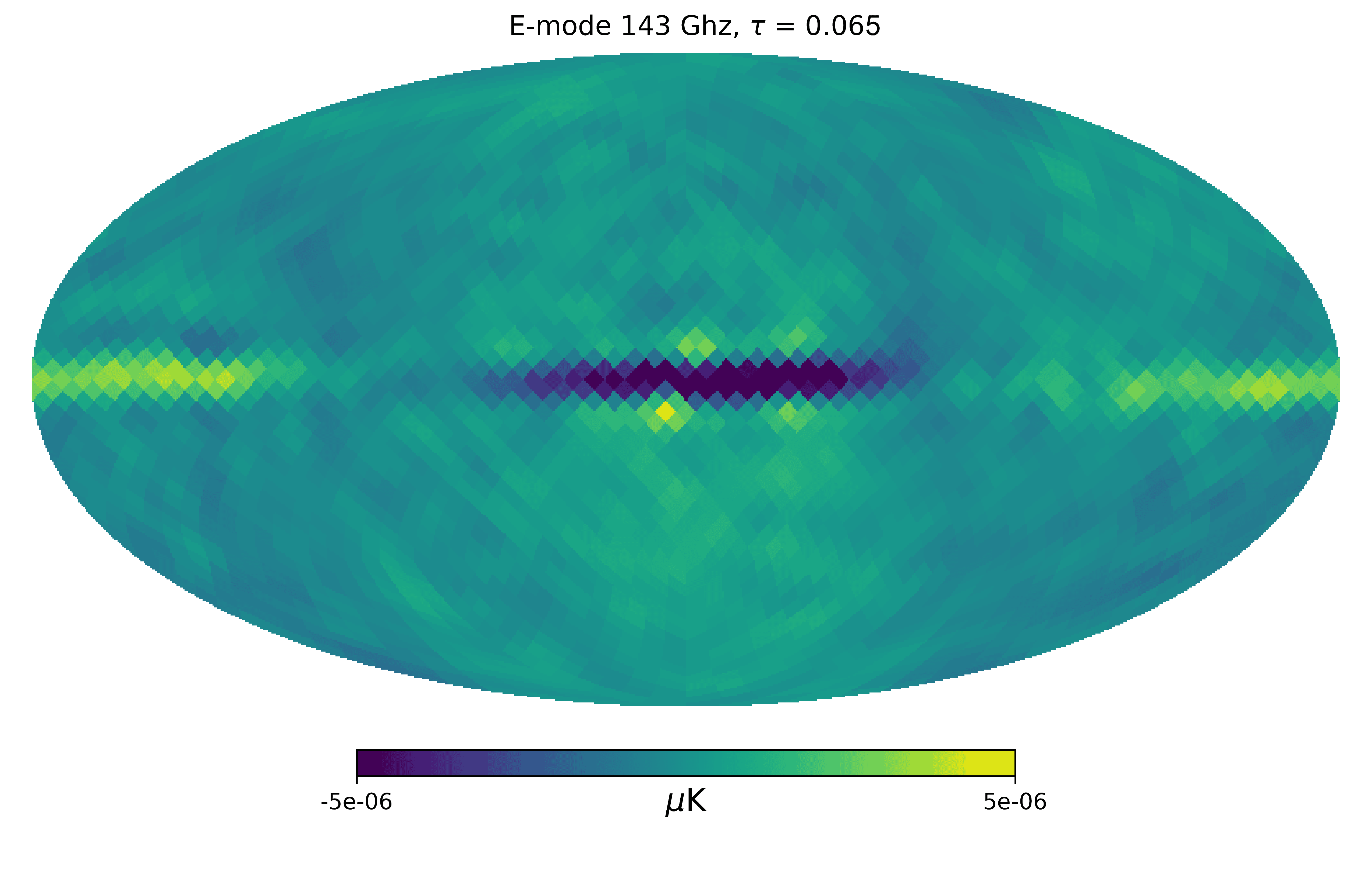
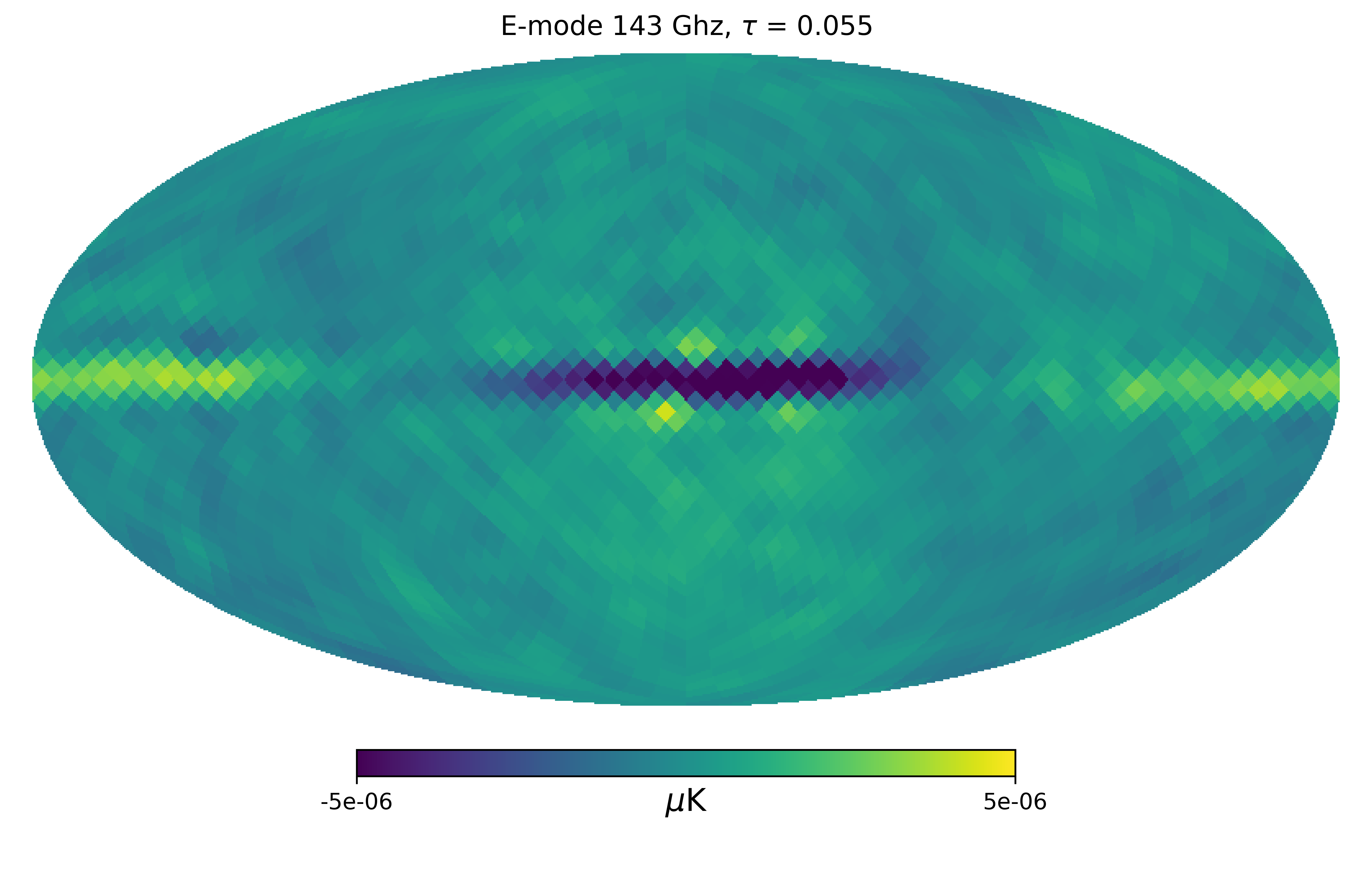
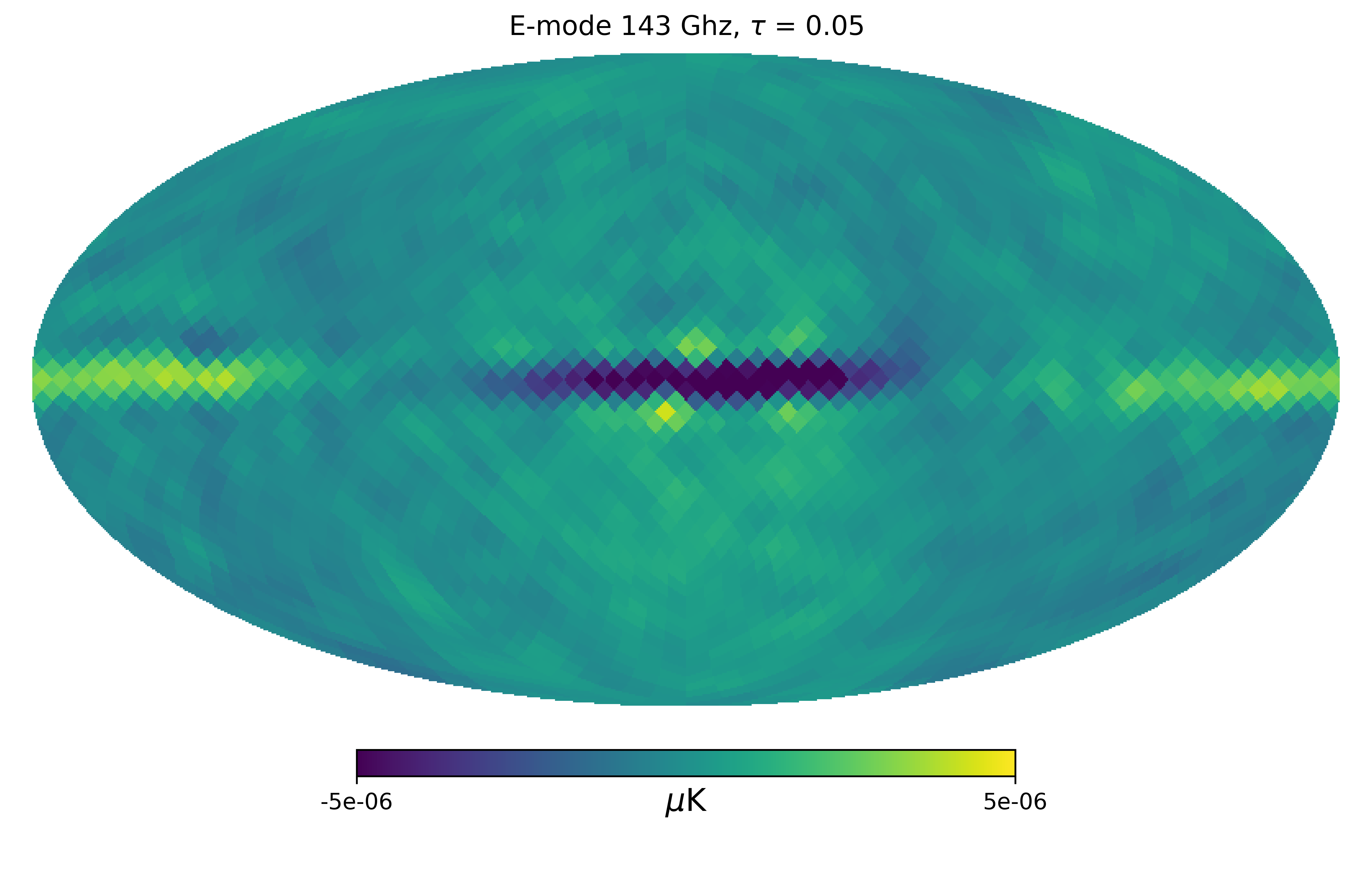
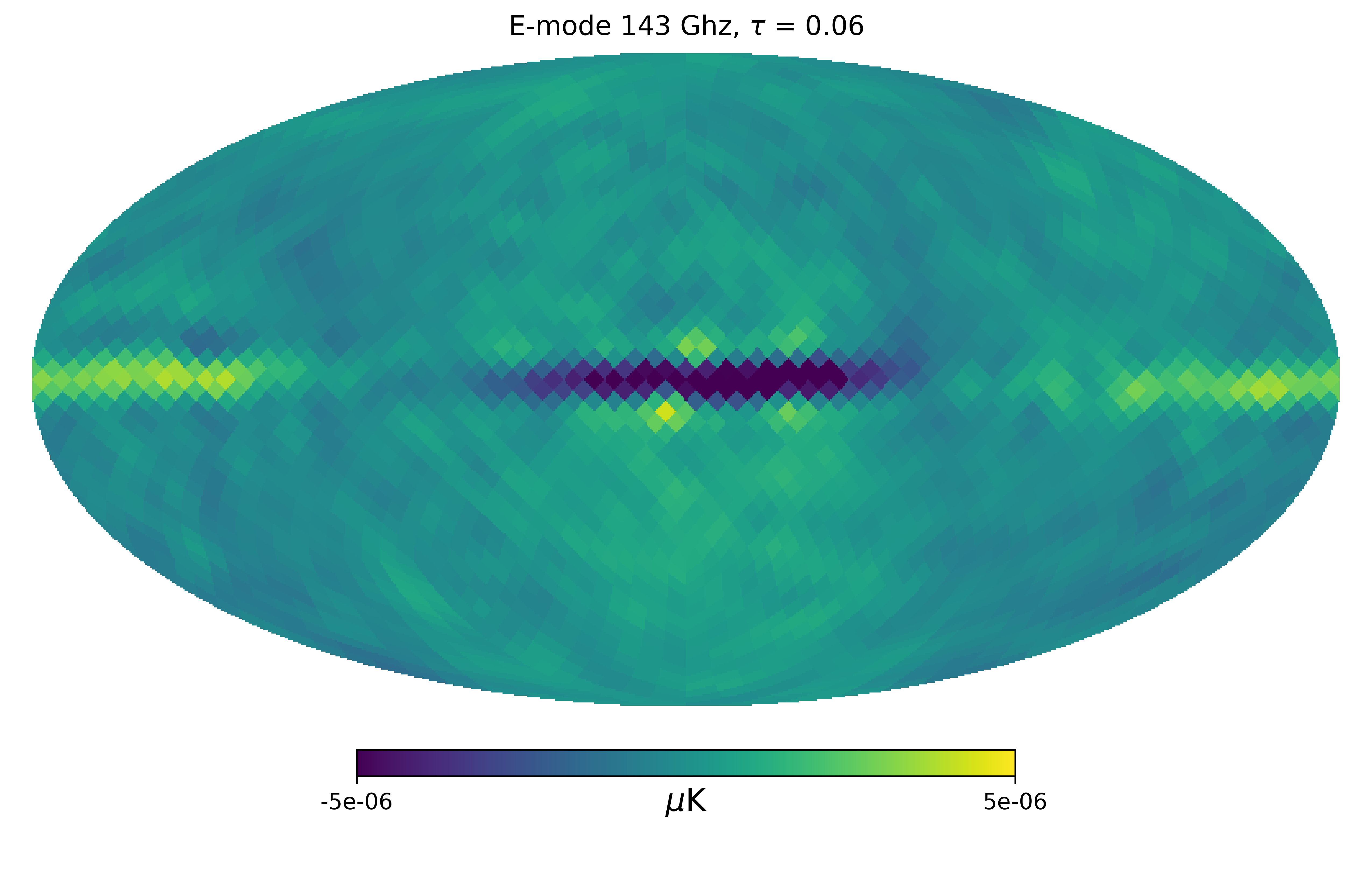
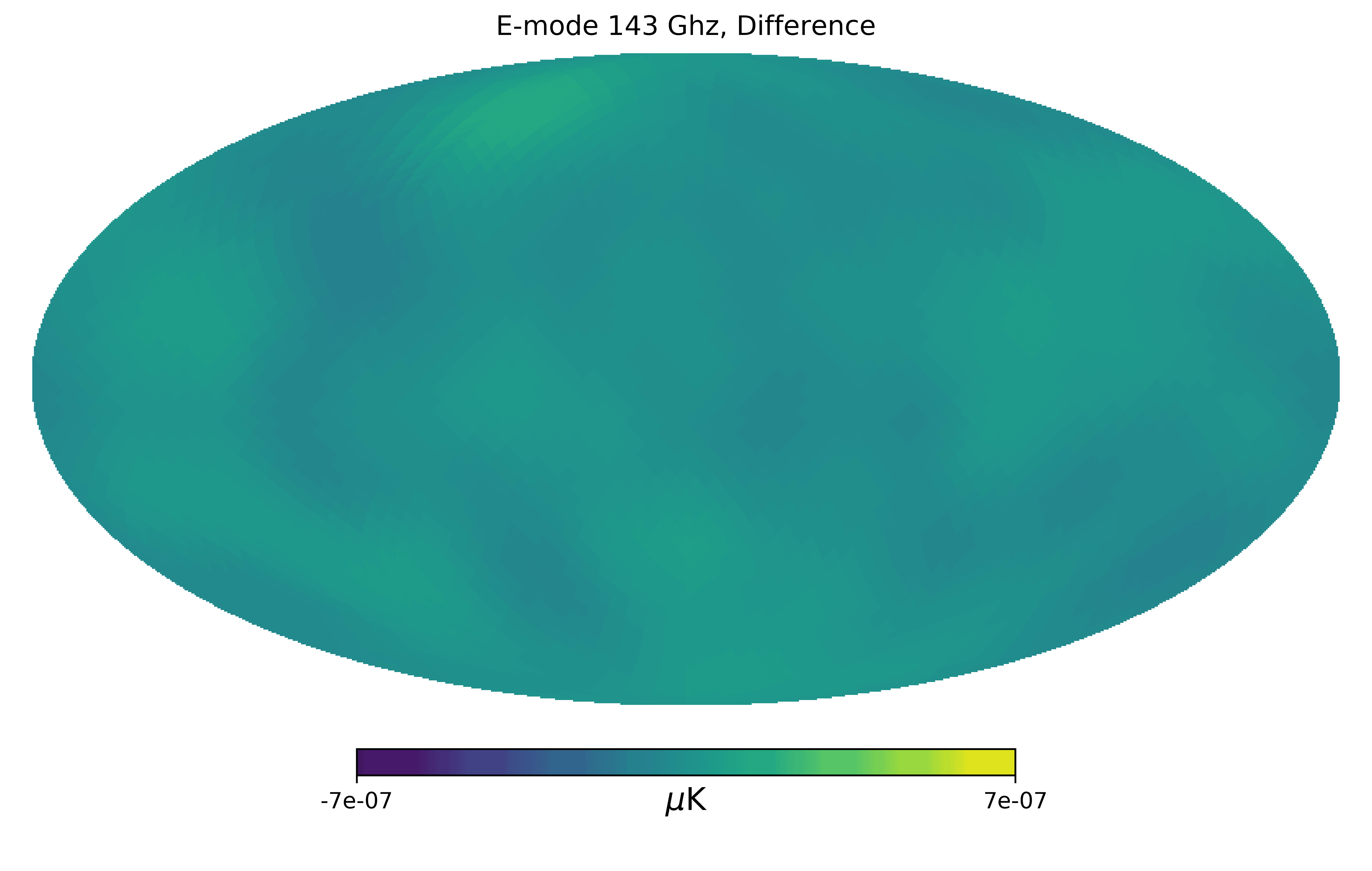
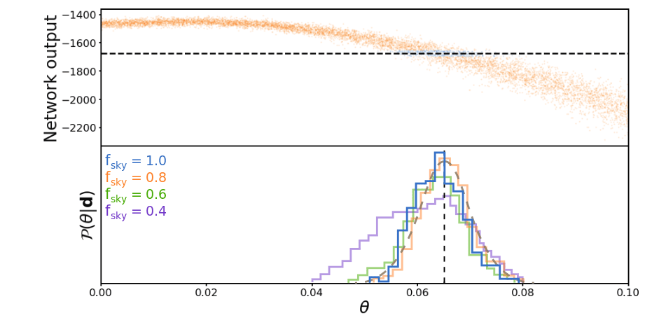
$\tau$ estimation from Planck E-mode polarisation maps¶

Use spherical convolutional neural network¶

We obtain a convincing posterior¶

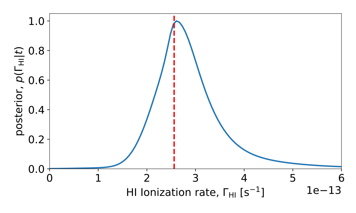
Inferring the ionisation rate from quasar absorption spectra¶

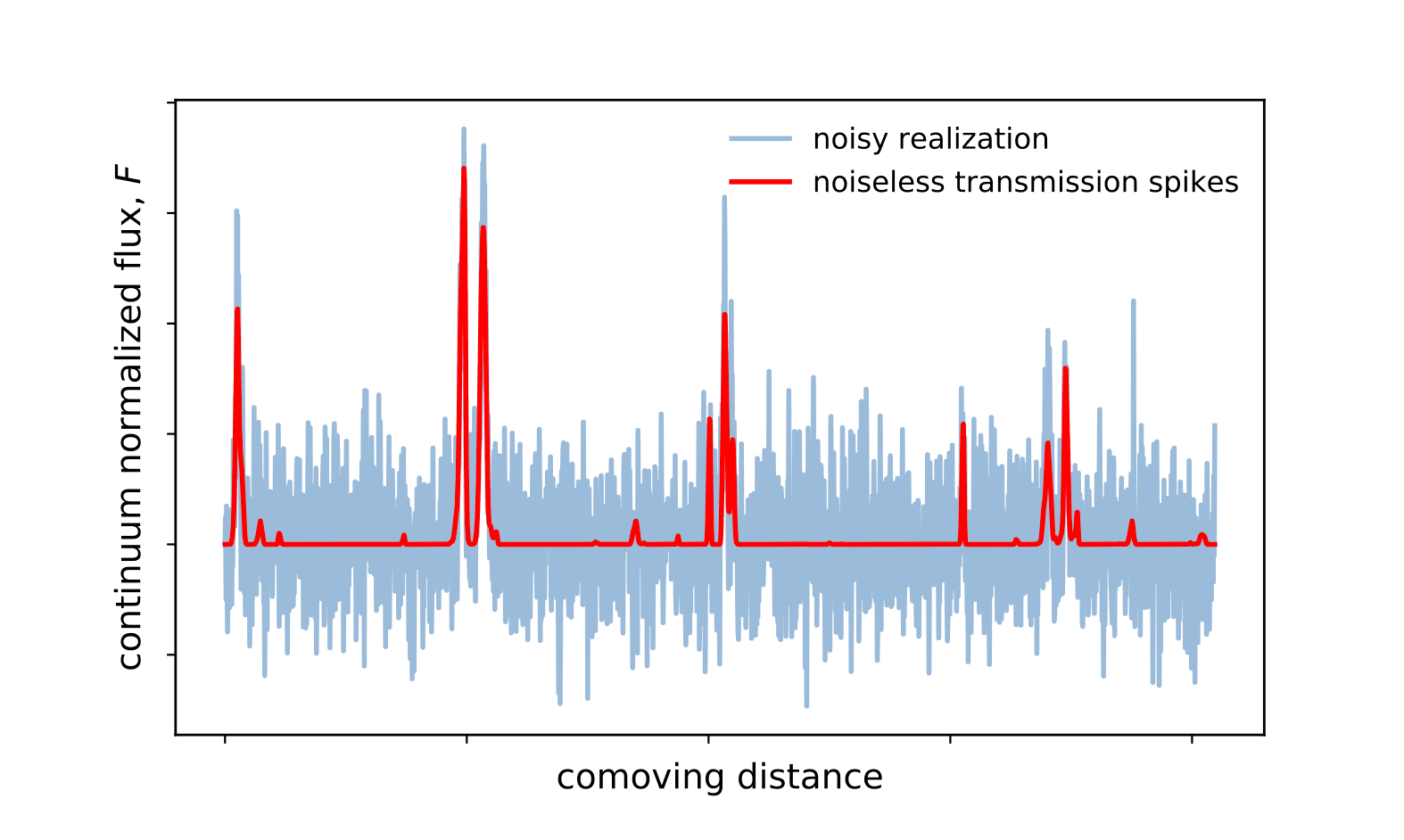
Use fully connected neural network¶

Couple it with DELFI to get another convincing posterior!¶

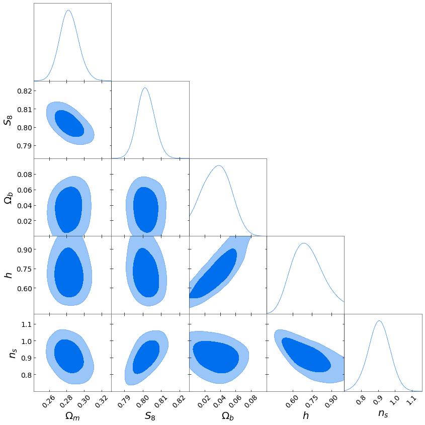
Multi-dimensional cosmological parameter inference from tomographic cosmic sheap maps of a Euclid-like survey¶

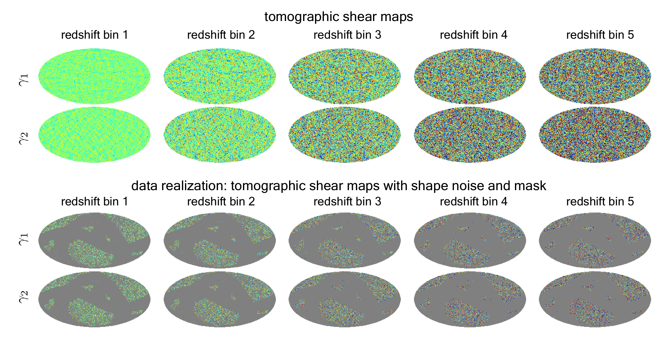
Summarise the maps via the power spectrum and compress that with the IMNN¶

Use DELFI for inference¶

Summary¶

Data must be compressed for us to effectively do ABC

Compression can be performed many different ways (although are most ways are lossy)

Score compression provides optimal summaries (which can be lossless if the likelihood is known)

IMNN enables us to transform data into Gaussian summaries which maximise all possible information

It's proving successful and we want to apply it to everything we can!

Download IMNN now!¶

pip install IMNN

github.com/tomcharnock/IMNN

For a bit of early morning compression fun why not run¶

Information maximising neural networks for dimensionality reduction¶

Dimensionality reduction¶

Data is big!¶

Even the number of summary statistics is $\sim$10$^\textsf{4}$!¶

Some (slightly) smaller simpler data¶

Why do we need data reduction?¶

Approximate Bayesian computation¶

ABC posterior¶

The curse of dimensionality¶

Inadequate sampling¶

Methods for dimensionality reduction¶

Informative compressed summaries¶

optimal compressed summaries¶

Fisher information¶

Expectation of the square of the score function at some fiducial model parameter values¶

How to build optimal compressed summaries¶

Use the score function as a set of summaries¶

The score function defines optimal compressed summaries¶

Informative compressed summaries¶

Linearly related to a maximum likelihood estimate¶

Great... but we're at a LIKELIHOOD-FREE inference workshop¶

We can try and approximate the likelihood¶

Can we be more general than this though?¶

Yes!¶

Information maximising neural networks¶

Load the (very easy to use) module¶

Non-linear compression function¶

So how do we find this magic function?¶

Find the function which gives Gaussian summaries¶

This function is a trained neural network¶

optimised to maximise the Fisher information!¶

Fisher information given our known Gaussian likelihood of summaries¶

Unbiased parameter estimate straight from the IMNN¶

Training the network¶

Build the network to best exploit the data¶

We can build the network to work on summaries with unknown likelihoods¶

Finding that one extra summary...¶

Of course we can still do score compression¶

Define our network¶

Generate training (and validation) data¶

Massively cheap¶

Let's build the IMNN¶

Pass $n_\textrm{sims}$ simulations through the network and calculate ${\bf C}_\mathscr{f}$¶

Calculate the derivative of the network outputs with respect to the parameters¶

Calculate the Fisher information¶

Update the network parameters using the gradient of the loss function¶

Lather, rince, repeat...¶

Do ABC (or similar)¶

How did we do (fingers crossed)¶

Examples¶

(and successes!)¶

$\tau$ estimation from Planck E-mode polarisation maps¶

Use spherical convolutional neural network¶

We obtain a convincing posterior¶

Inferring the ionisation rate from quasar absorption spectra¶

Use fully connected neural network¶

Couple it with DELFI to get another convincing posterior!¶

Multi-dimensional cosmological parameter inference from tomographic cosmic sheap maps of a Euclid-like survey¶

Summarise the maps via the power spectrum and compress that with the IMNN¶

Use DELFI for inference¶

Summary¶

Download IMNN now!¶