Neural physical engines for inferring the halo mass distribution function¶

Tom Charnock

Institut d'Astrophysique de Paris

Notebook: presentations.charnock.fr/NPE

Cosmology from the universe¶

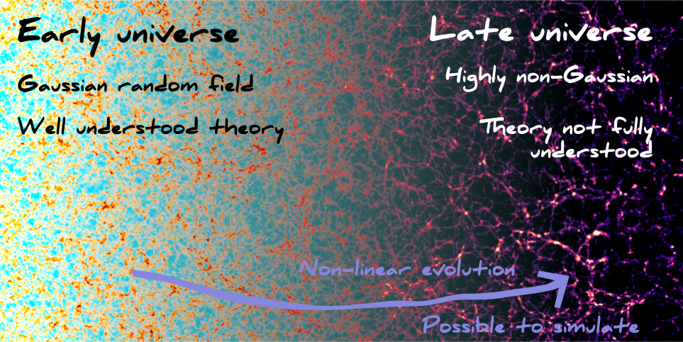
Bayesian Origins Reconstruction of Galaxies (BORG)¶

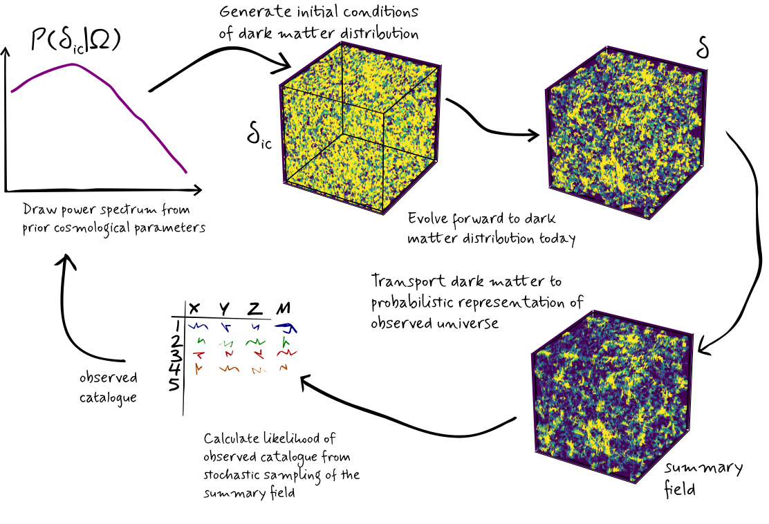
Infer the dark matter field from any catalogue¶

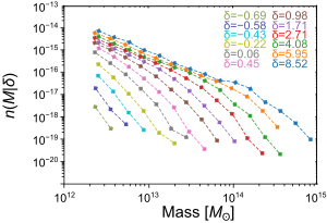
Halo mass distribution function¶

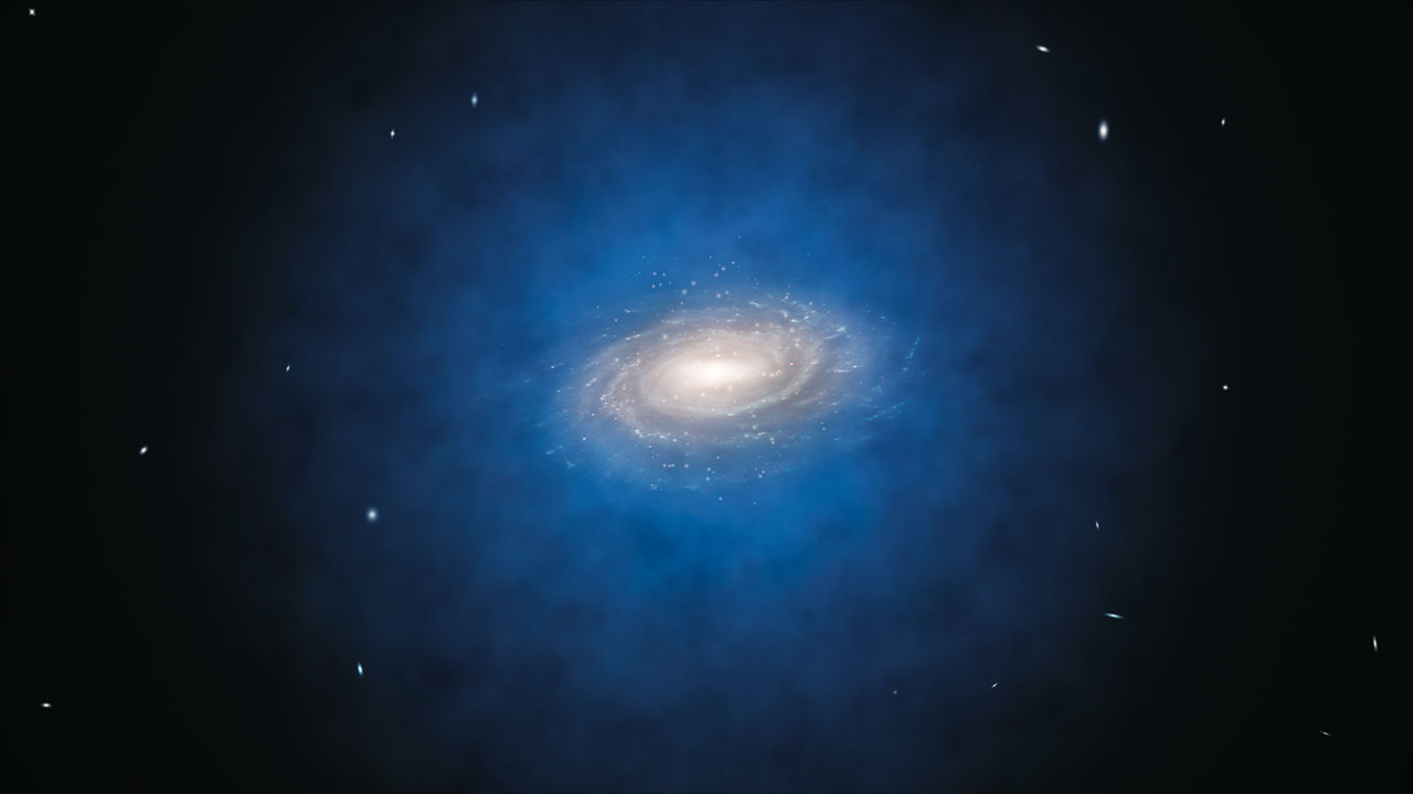
Distribution of halos¶

Press Schechter (gravitational collapse following power law at small masses, exponential cut-off)
Local density deviations
Unknown stochasticity (Poissionian)

Halo mass distribution¶

Neural bias model¶

_{github:neural_bias_model}

Neural physical engines¶

Build networks using physical principles.

Reduces number of parameters
Increases computational efficiency
Decreases overfitting
Improves interpretability

Convolutions for translational invariance¶

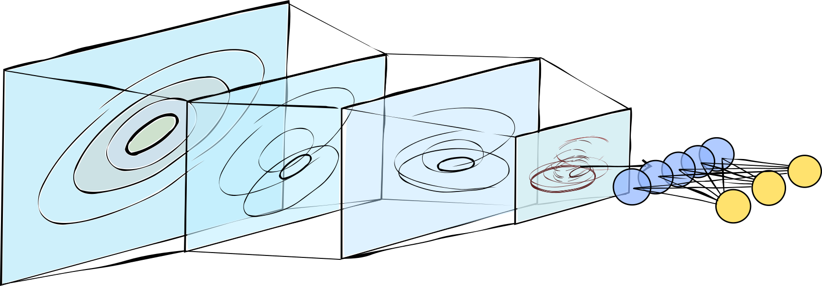
Architecture suited to the data¶

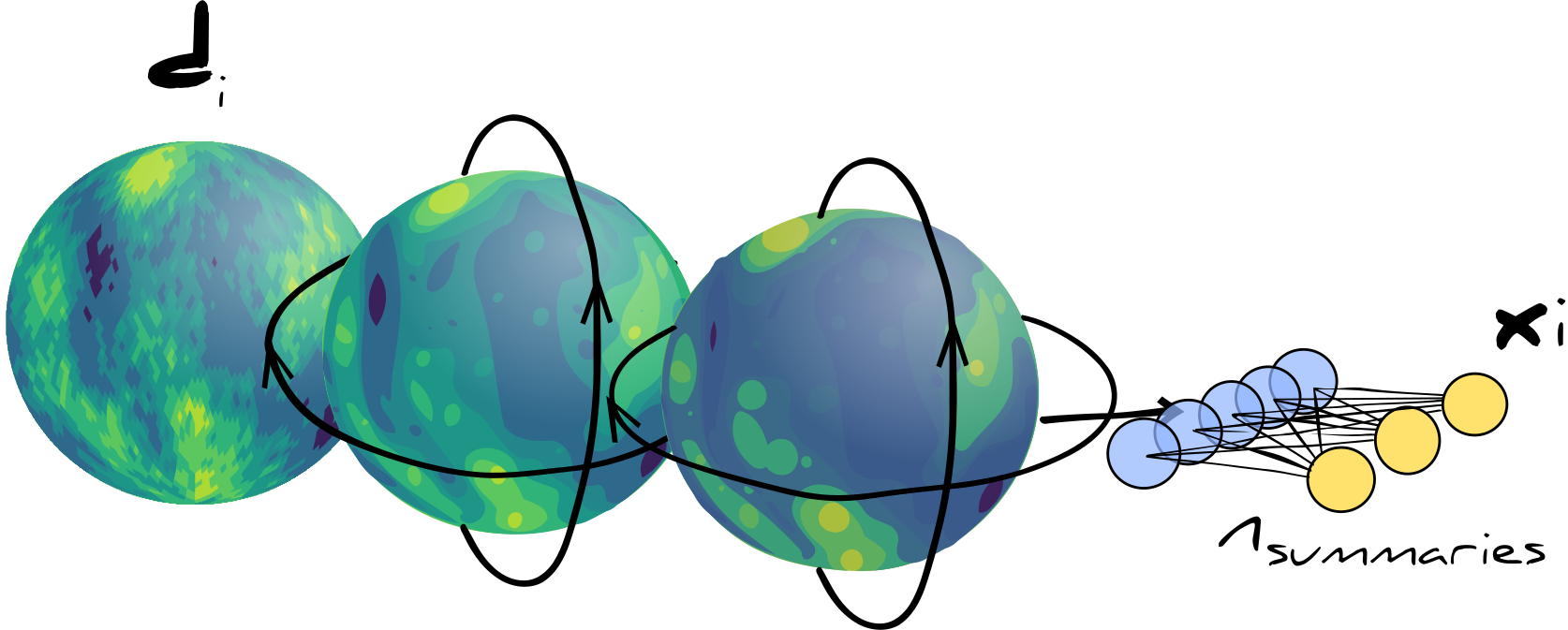
Use only causally relevant features¶

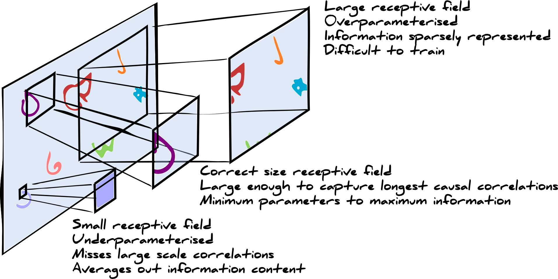
Use only informative features¶

_{github:multipole_kernels}

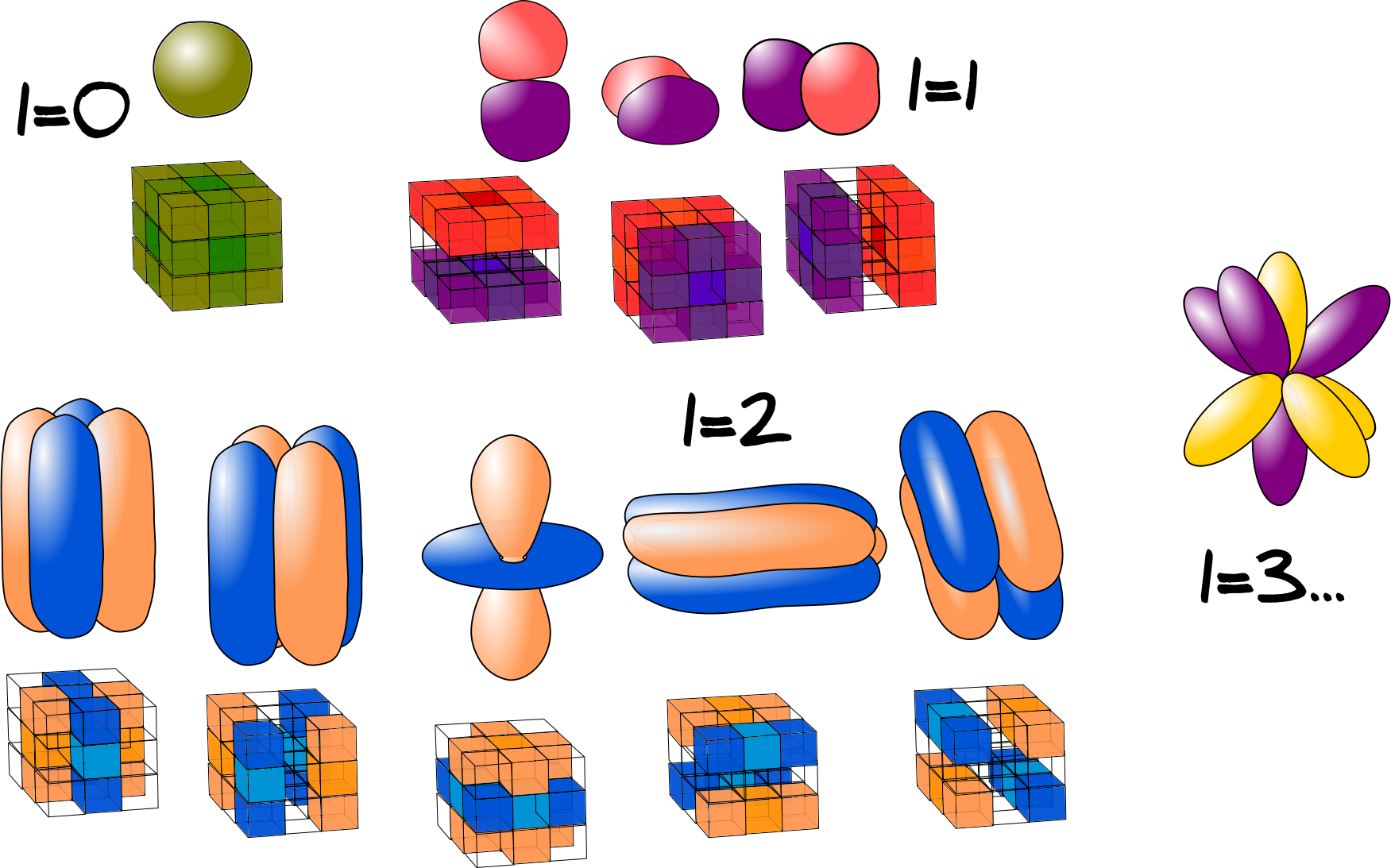
What's the best map from the dark matter density today to some summary of the halos?¶

We don't actually know yet...¶

We do know that it should be:¶

Dependent on the local patch
Mostly sensitive to the amplitude
Independent of position on the sky

Our neural physical engine¶

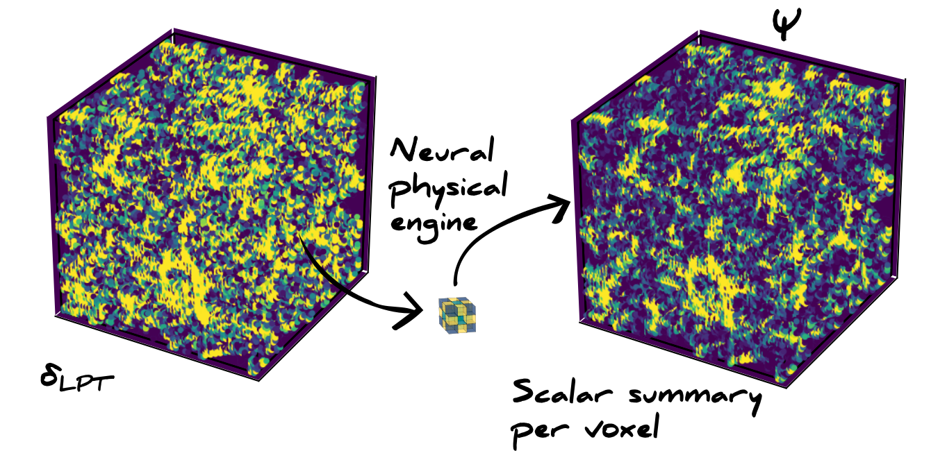
$${\Tiny \psi_j^{\ell,m} = A\left(\sum_{i=-\kappa/2}^{i=\kappa/2}K_{i}^{\ell,m}\delta_{j-i}^\textrm{LPT}+b_j\right), ~~~ \ell=0, m=0}$$

Neural density estimators¶

Halo mass distribution function is a smooth function of mass given a density environment¶

Use a mixture density network¶

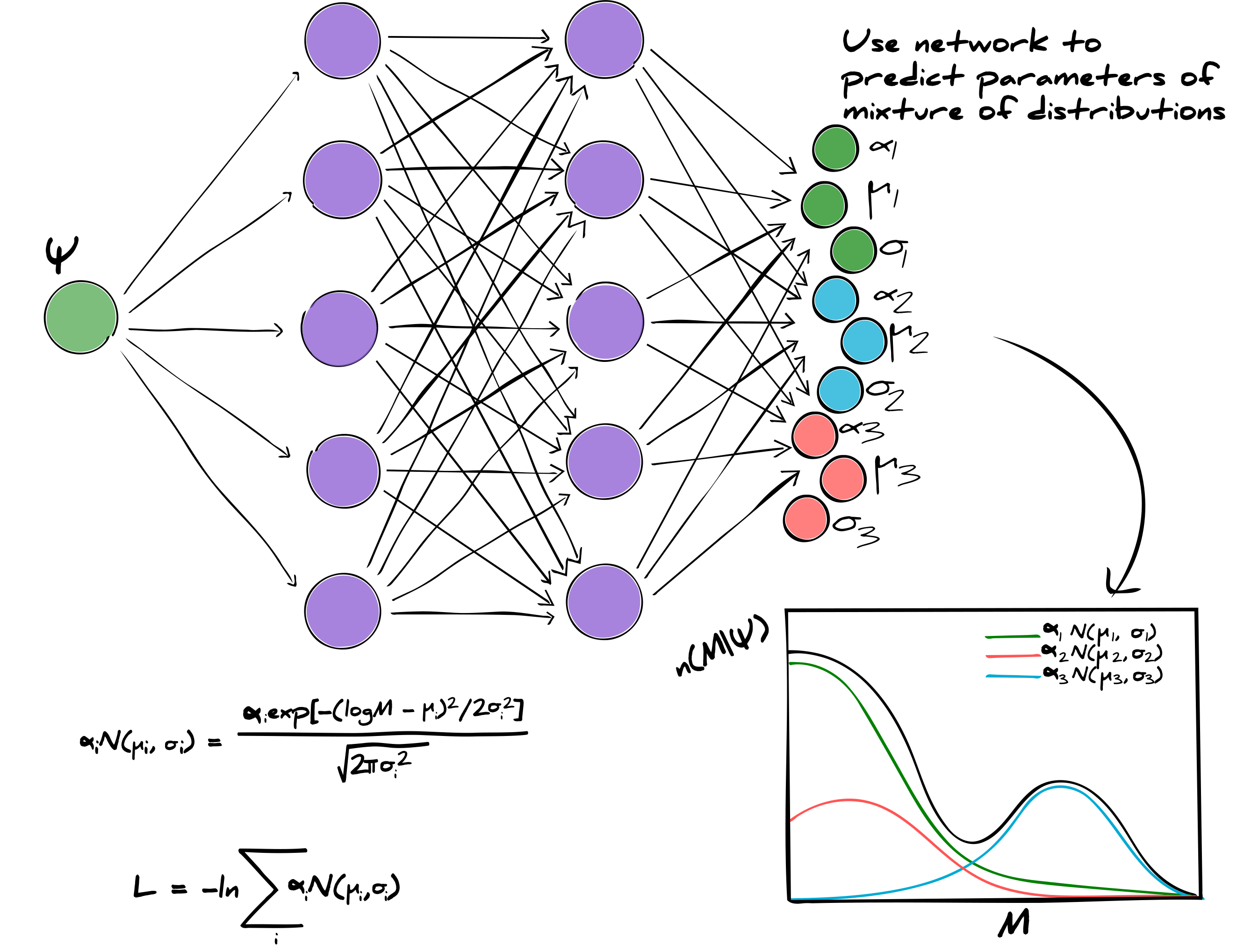
Our neural density estimator¶

$$\begin{align*} {\tiny n(M|\delta) =}&{\tiny \sum_i^N\alpha(\boldsymbol{\psi}, \boldsymbol{\theta}_i^{\boldsymbol{\alpha}})\mathcal{N}\left(\mu(\boldsymbol{\psi}, \boldsymbol{\theta}_i^{\boldsymbol{\mu}}), \sigma(\boldsymbol{\psi}, \boldsymbol{\theta}_i^{\boldsymbol{\sigma}})|M\right),}\\ {\tiny =}&{\tiny \sum_i^N\frac{\alpha(\boldsymbol{\psi}, \boldsymbol{\theta}_i^{\boldsymbol{\alpha}})}{\sqrt{2\pi\left(\sigma(\boldsymbol{\psi}, \boldsymbol{\theta}_i^{\boldsymbol{\sigma}})\right)^2}}\exp\left[-\frac{\left(\log(M) - \mu(\boldsymbol{\psi}, \boldsymbol{\theta}_i^{\boldsymbol{\mu}})\right)^2}{2\left(\sigma(\boldsymbol{\psi}, \boldsymbol{\theta}_i^{\boldsymbol{\sigma}})\right)^2}\right],}\end{align*} $$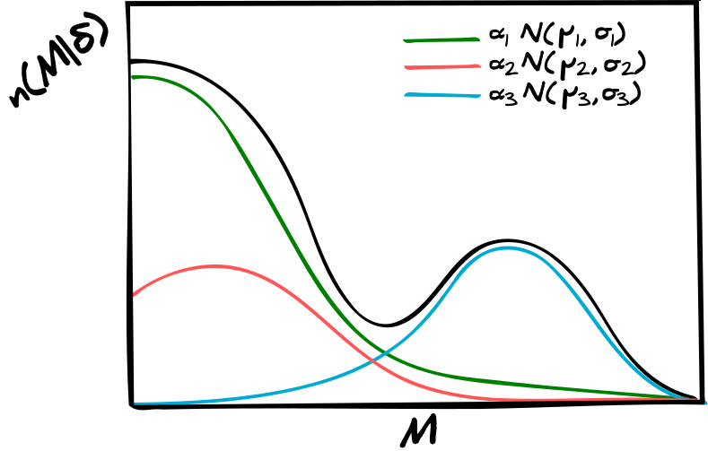

$$ \begin{align*} {\tiny\alpha_i} & {\tiny=\text{softplus}(w_{i}^\alpha\boldsymbol{\psi}+b^\alpha_i),}\\ {\tiny\mu_i }&{\tiny = \left\{\begin{array}{ll} w_{i}^\mu\boldsymbol{\psi}+b^\mu_i&i=0\\ \textrm{Max}\left[0,~ w_{i}^\mu\boldsymbol{\psi}+b^\mu_i\right]+\mu_{i-1}&i>0\\ \end{array}\right.,}\\ {\tiny\sigma_i} &{\tiny = \text{softplus}(w_{i}^\sigma\boldsymbol{\psi}+b^\sigma_i)\;,} \end{align*} $$

_{2 Gaussians with
${\Tiny\boldsymbol{b}^\alpha \to \boldsymbol{b}^\alpha +\log(10^{-3})}$, ${\Tiny b_0^\mu \to b_0^\mu + \log\left(2\times10^{12}\right)}$ and ${\Tiny\boldsymbol{b}^\sigma\to \boldsymbol{b}^\alpha + \log(10^3)}$.}

Likelihood¶

$$\begin{align*} {\Tiny\mathcal{L} =}&{\Tiny \sum_{j\in\textrm{catalogue}}\log\left[\sum_i^N\frac{\alpha_{i,j}}{\sqrt{2\pi\sigma_{i,j}^2}}\exp\left[-\frac{\left(\log(M_j) - \mu_{i,j}\right)^2}{2\sigma_{i,j}^2}\right]\right]}\\ &{\Tiny - V\sum_{j\in\textrm{voxels},i=1}^N\frac{\alpha_{i,j}}{2}\exp\left[\frac{\sigma_{i,j}^2}{2}\right]\textrm{erfc}\left[\frac{\log\left(M_\textrm{th}\right) - \mu_{i,j} - \sigma_{i,j}^2}{\sqrt{2\sigma_{i,j}^2}}\right].} \end{align*}$$

This is Poissonian.
But on the NPE field, so it is non-local

HMCLET¶

We want to infer the weights of the neural bias model¶

Hamiltonian Monte Carlo¶

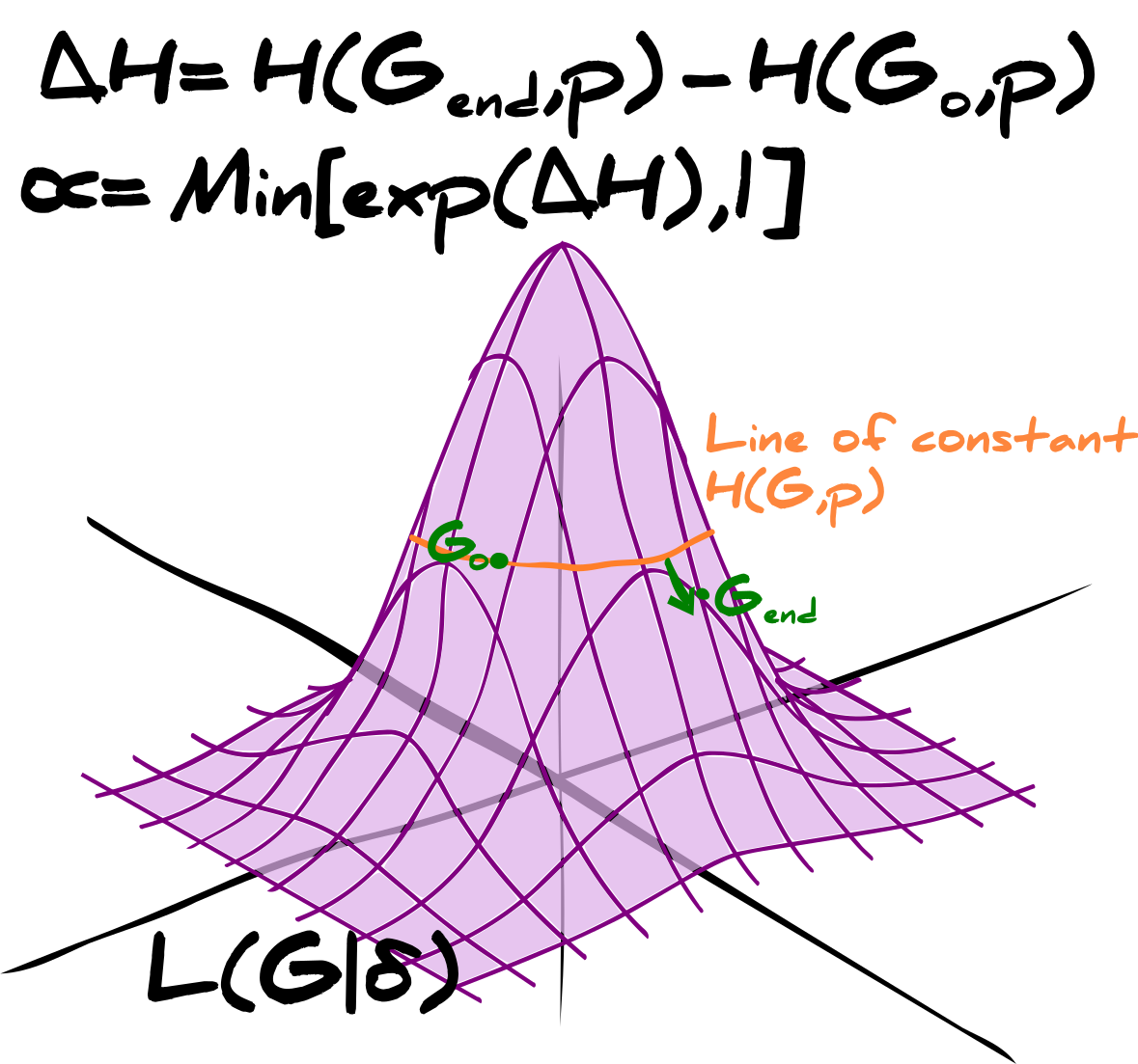
_{Introduce momentum ${\small {\bf p}\leftarrow\mathcal{N}({\bf 0},{\bf M})}$ and solve Hamilton's equations}

$$\begin{align*} {\Tiny\mathcal{H}(\boldsymbol{\theta}, {\bf p}) }&{\Tiny~= \mathcal{V}(\boldsymbol{\theta}) + \mathcal{K}({\bf p})}\\ &{\Tiny~=\mathcal{L}(\boldsymbol{\theta}|\boldsymbol{\delta})-\log\left[\pi(\boldsymbol{\theta})\right]+\frac{1}{2}{\bf p}^T{\bf M}^{-1}{\bf p}} \end{align*}$$ _{Accept samples according to probability} $$\begin{equation*} {\Tiny\alpha = \textrm{Min}\left[\exp\left(\Delta\mathcal{H}\right), 1\right]} \end{equation*}$$

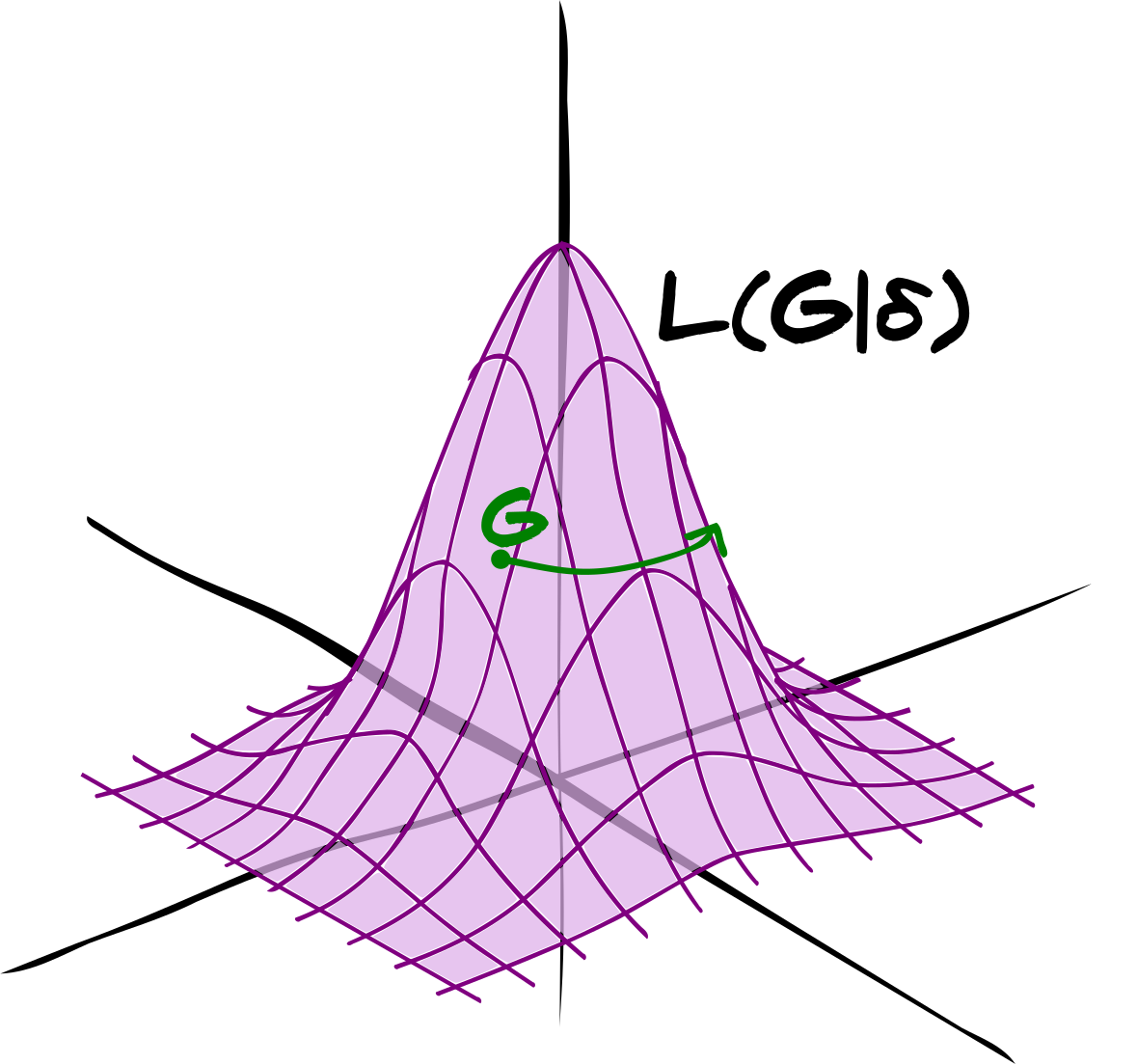
Evolve using ${\Tiny\dot{\boldsymbol{\theta}}= {\bf M}^{-1}{\bf p}}$ and ${\Tiny\dot{\bf p}= -\nabla\mathcal{V}(\boldsymbol{\theta})}$

Acceptance is guaranteed if ODEs are perfectly solved¶

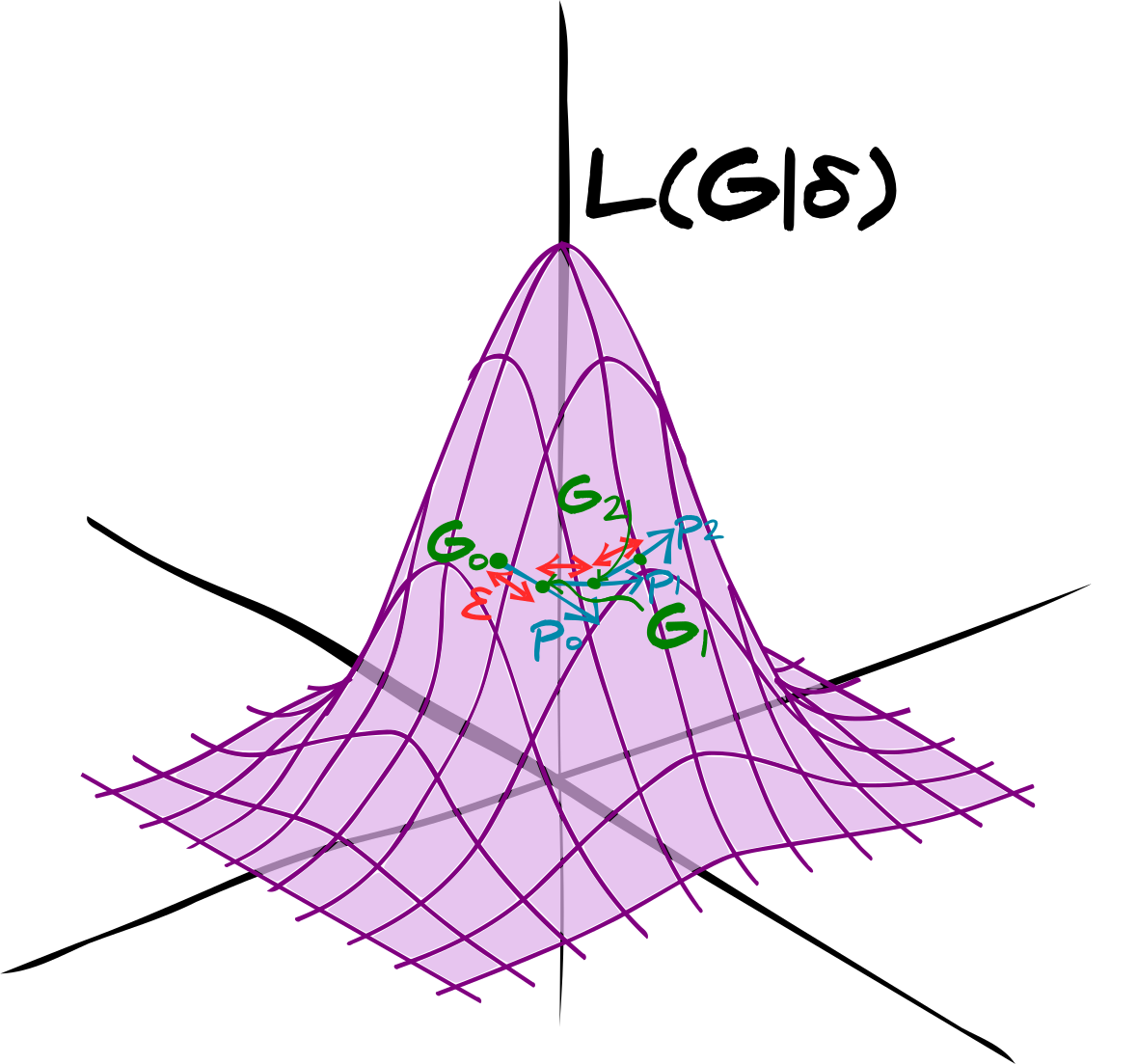
Use leapfrog algorithm¶

Leapfrog algorithm¶

Acceptance criterion¶

How does this work for neural networks?¶

Likelihood surface is extremely flat and highly degenerate¶

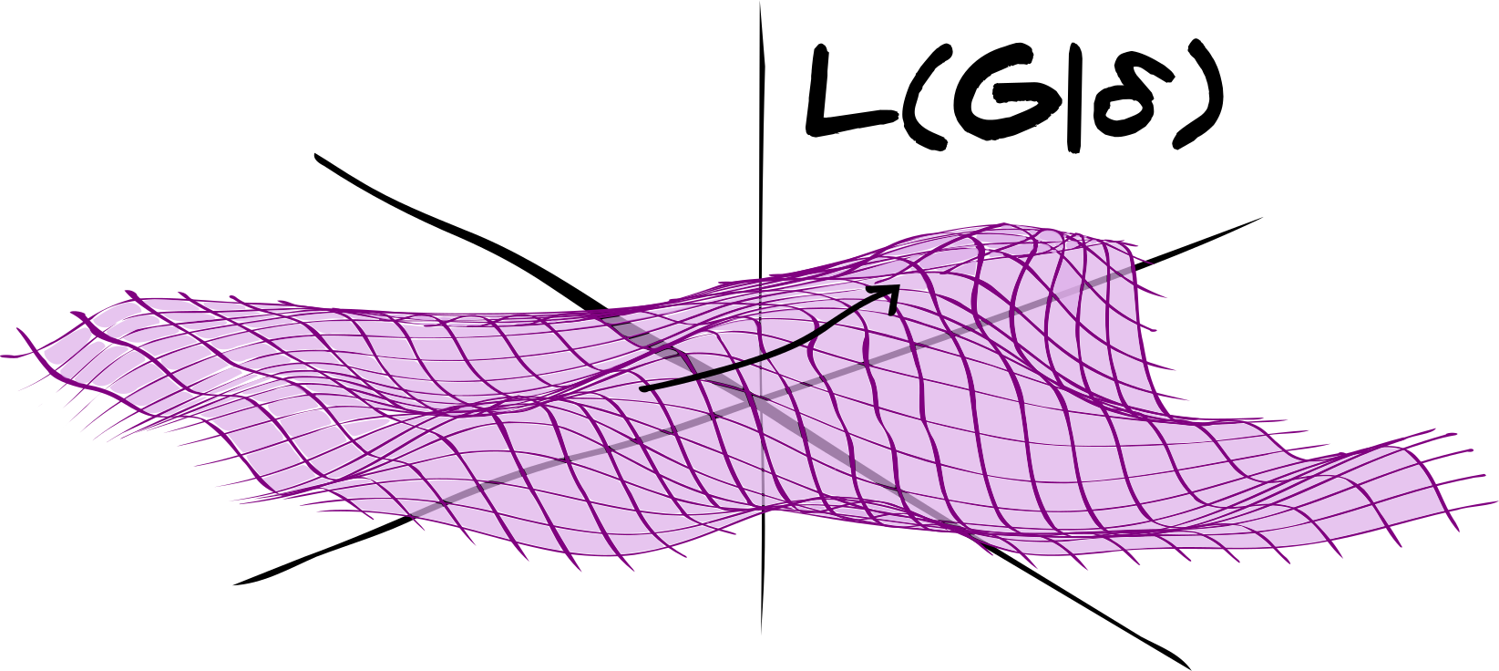
Nearly impossible to know the mass matrix, ${\bf M}$.

Use second order geometric information¶

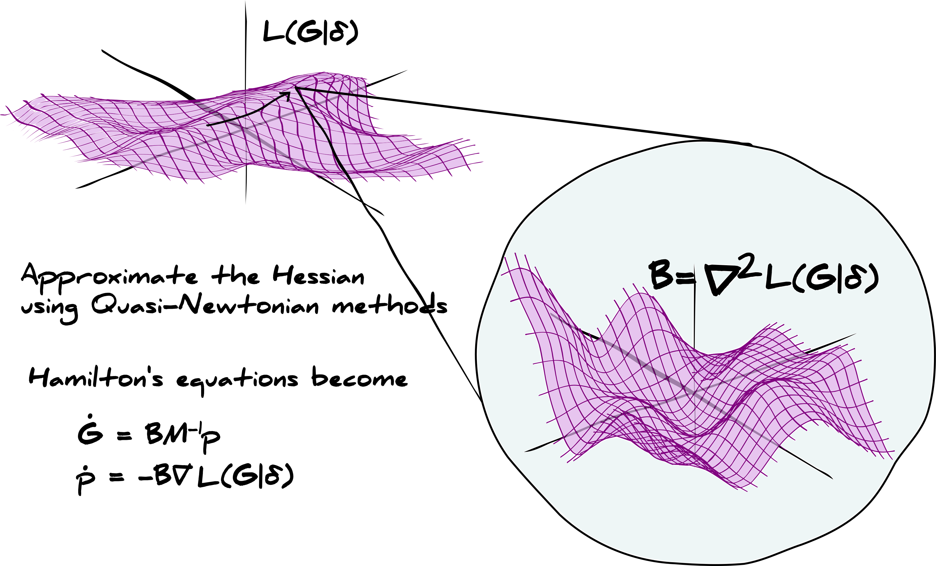
Quasi-Newtonian inverse Hessian¶

$$\begin{equation*} {\Tiny{\bf B}^*=\left(\mathbb{I}-\frac{\boldsymbol{s}_i\boldsymbol{y}_i^T}{\boldsymbol{y}_i^T\boldsymbol{s}_i}\right){\bf B}_i\left(\mathbb{I}-\frac{\boldsymbol{y}_i\boldsymbol{s}_i^T}{\boldsymbol{y}_i^T\boldsymbol{s}_i}\right)+\frac{\boldsymbol{s}_i\boldsymbol{s}_i^T}{\boldsymbol{s}_i^T\boldsymbol{y}_i},} \end{equation*} $$

_{with ${\Tiny\boldsymbol{s}_i=\boldsymbol{\theta}^*-\boldsymbol{\theta}_i}$ and ${\Tiny\boldsymbol{y}_i=\nabla\mathcal{L}(\boldsymbol{\theta}^*|\boldsymbol{\delta})-\nabla\mathcal{L}(\boldsymbol{\theta}_i|\boldsymbol{\delta})}$.}

Both $\boldsymbol{s}$ and $\boldsymbol{y}$ come for free with the leapfrog algorithm¶

We can now successfully traverse the likelihood surface¶

The momenta and trajectories get rescaled by the Hessian providing a surface which is not as highly degenerate or flat

Actual results¶

VELMASS simulation¶

125h^-1Mpc chunk from 2h^-1Gpc length box
Rebinned to 64³ voxels
Planck-like cosmology
Halos found using Rockstar ~ O(10⁴) halos
Minimum halo size of 8x10⁸ solar masses

Run BORG¶

Sample the power spectrum¶

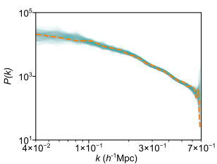✓ Power spectra remain smooth and close to prior

Sample the weights of the neural bias model¶

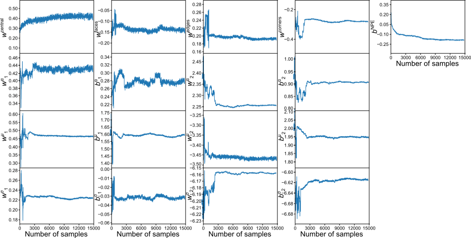
✓ Weight values are properly sampled after burn in
✓ NPE acts as a contrast enhancer

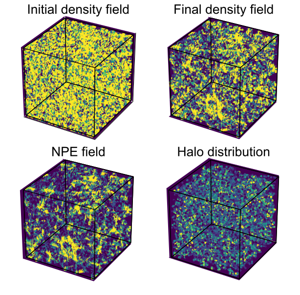
See the effects of the neural physical engine¶

✓ Non-local information is used to improve fit

And what does the halo mass distribution function look like?¶

Halo mass distribution function from neural bias model¶

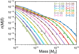✓ Fits data!

Conclusions¶

First example of zero-shot training, fully Bayesian neural network¶

Using neural physical engines to keep number of parameters small
Using the HMCLET to sample the weights of the neural network even though the likelihood is flat and degenerate
Using BORG to infer the simulations

Future work¶

Skip the bias completely by flowing the dark matter distribution to the stochastically sampled data (inferring the likelihood)
Optimisation of the neural physical engine architecture for optimal halo mass distribution function

Neural physical engines for inferring the halo mass distribution function¶

Tom Charnock

Institut d'Astrophysique de Paris

In [ ]: