Novel uses of machine learning:
Predicting probabilities and trusting outputs
Tom Charnock
Institut d'Astrophysique de Paris
Notebook: presentation.charnock.fr/ED

|

|
|

|
|
Who am I?
Tom Charnock
- Stastistican
- Cosmologist
- Machine learning safety and interpretability enthusiast
- TensorFlow fan
Cool things I've done with machine learning
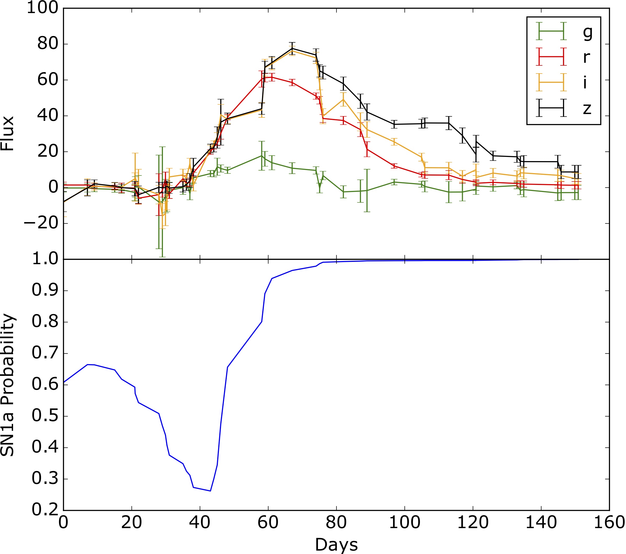
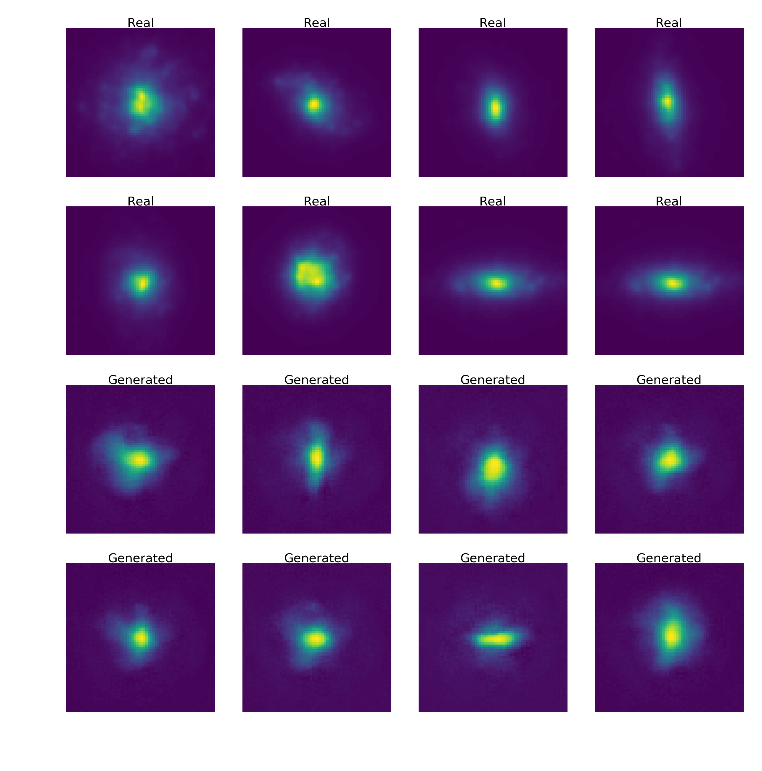
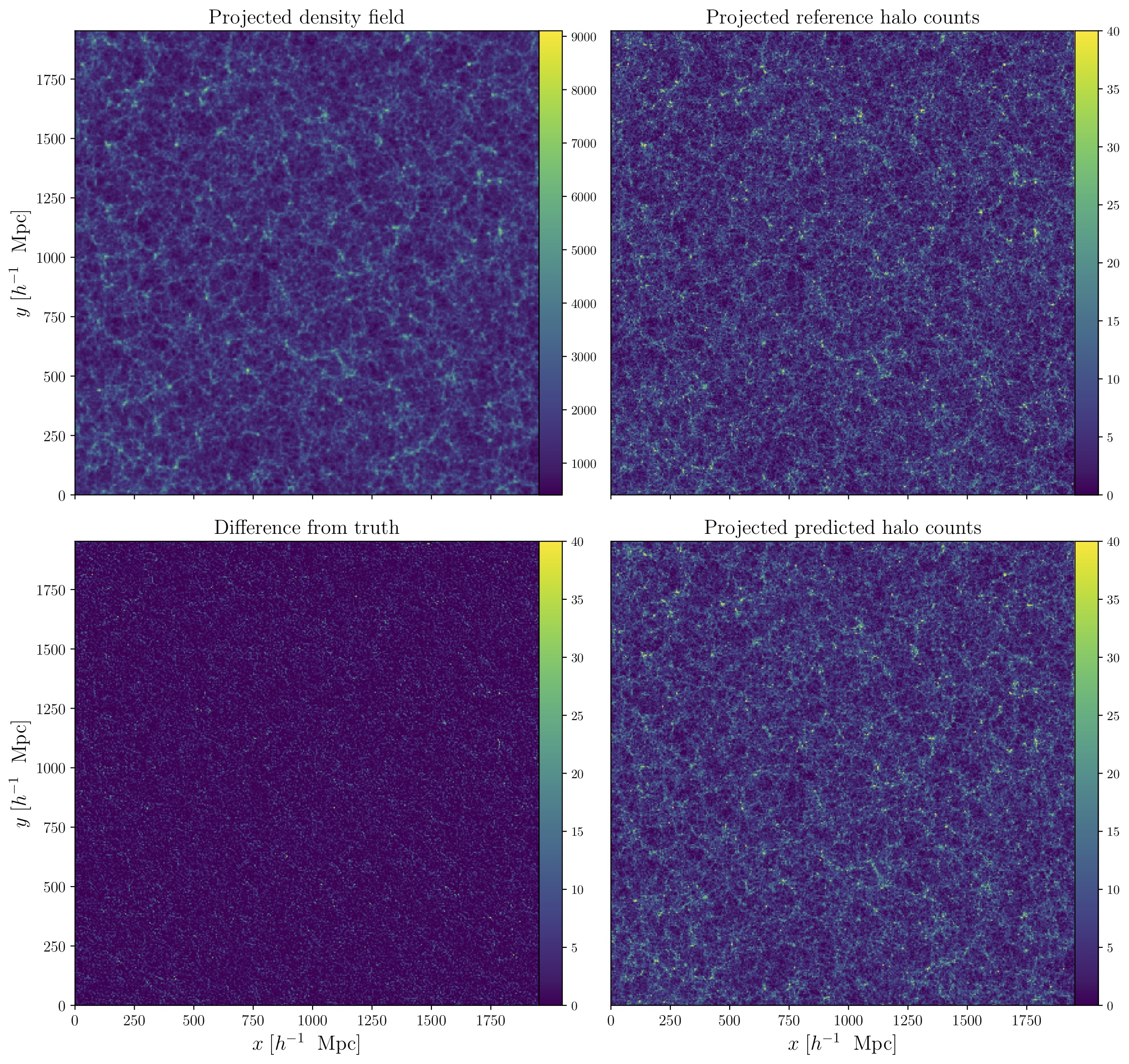
Physically motivated mapping networks (this week)
WGAN-like training algorithm
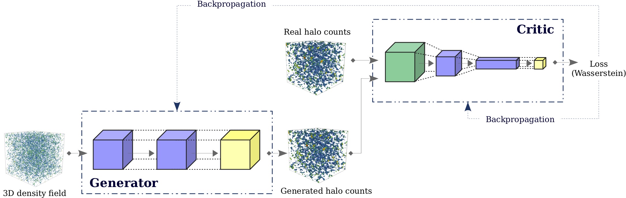
Generator maps known distribution to some physically related quantity
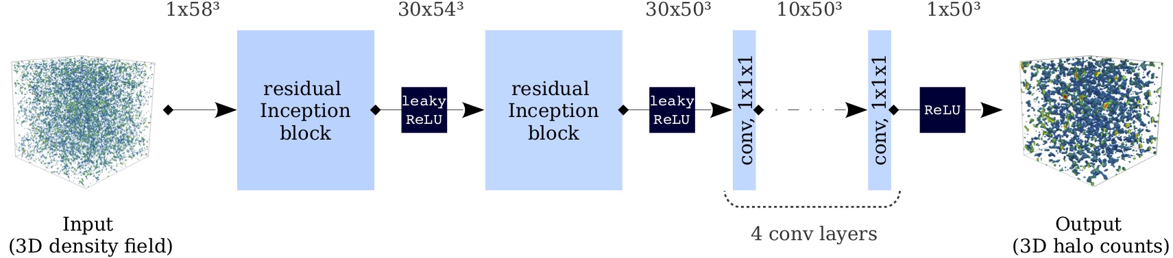
Architecture chosen to pull out physical intution
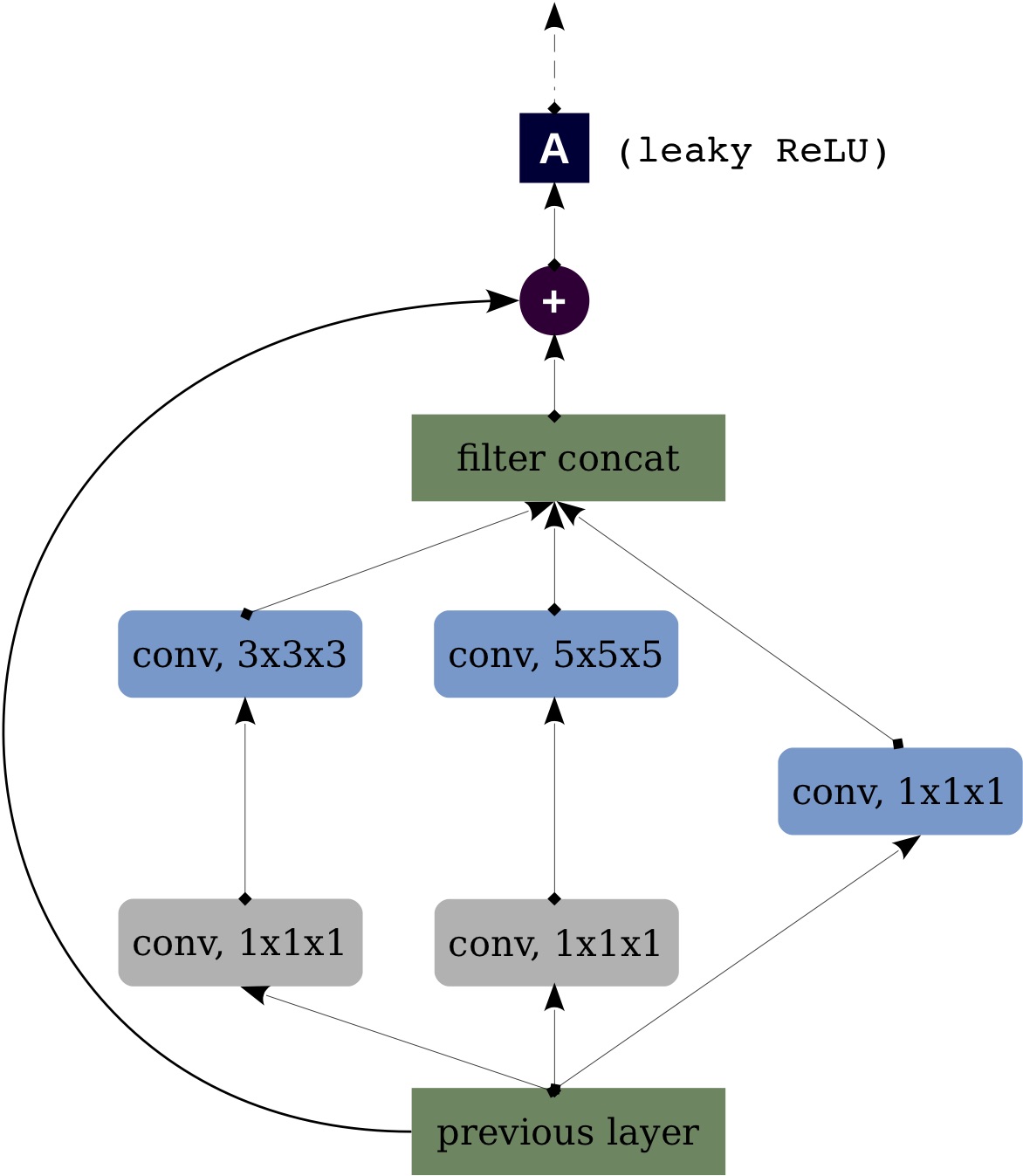
Need a critic which is able to be informative on the physical scale of relevance
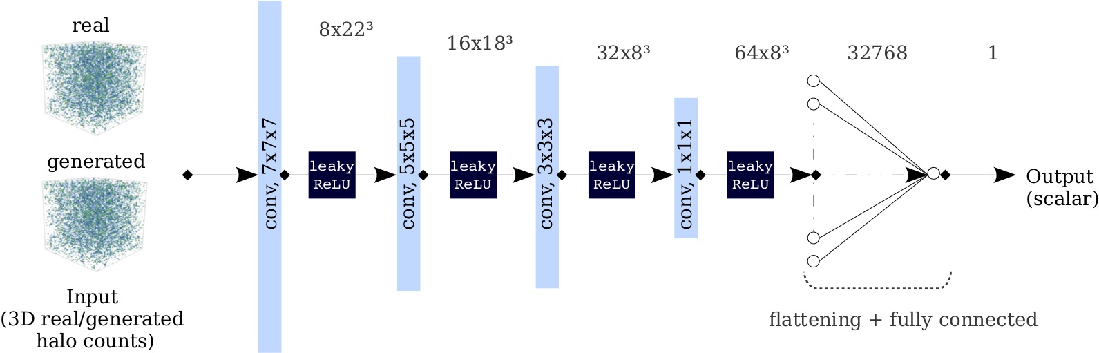
- Generate simulation
- Pass simulation and real data through critic
- Update weights of critic until converged (approx. Wasserstein)
- Fix critic weights
- Single update of the generator
Neural density estimators
Stats time
Data ${\bf d}$ described by parameters $\boldsymbol{\theta}$ with likelihood $\mathcal{L}({\bf d}|\boldsymbol{\theta})$
Posterior of parameters $\boldsymbol{\theta}$ found using Bayes theorem
$$\mathcal{P}(\boldsymbol{\theta}|{\bf d})=\frac{\mathcal{L}({\bf d}|\boldsymbol{\theta})p(\boldsymbol{\theta})}{p({\bf d})}$$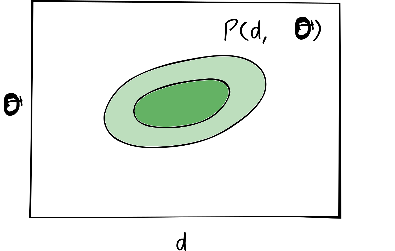
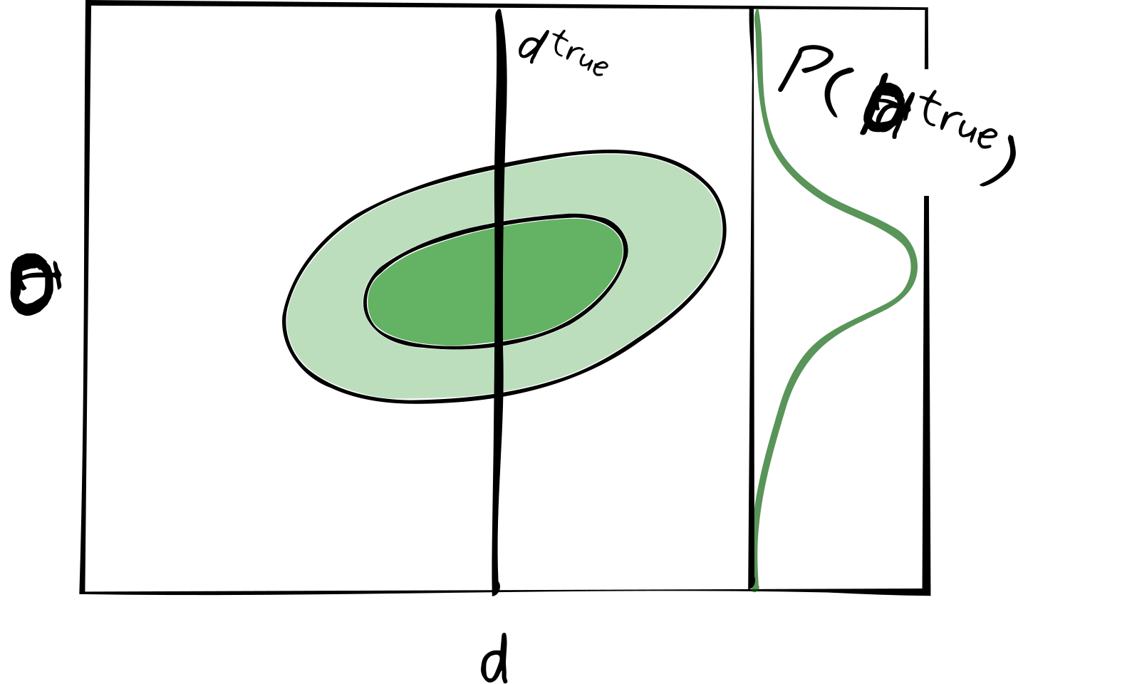
We can use NDEs to approximate
$\mathcal{P}(\boldsymbol{\theta}|{\bf d})$
Mixture density networks
Any function* can be approximated with a mixture of distributions
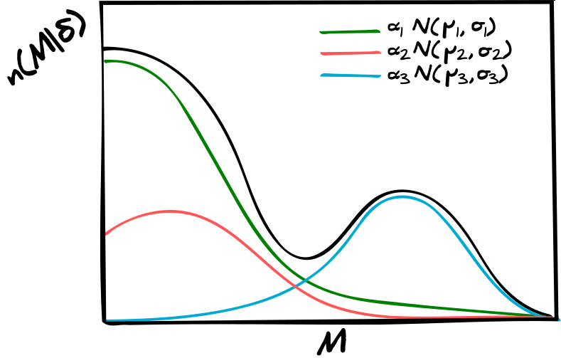
*under certain conditions
We can simply fit the parameters of the distributions using regression!
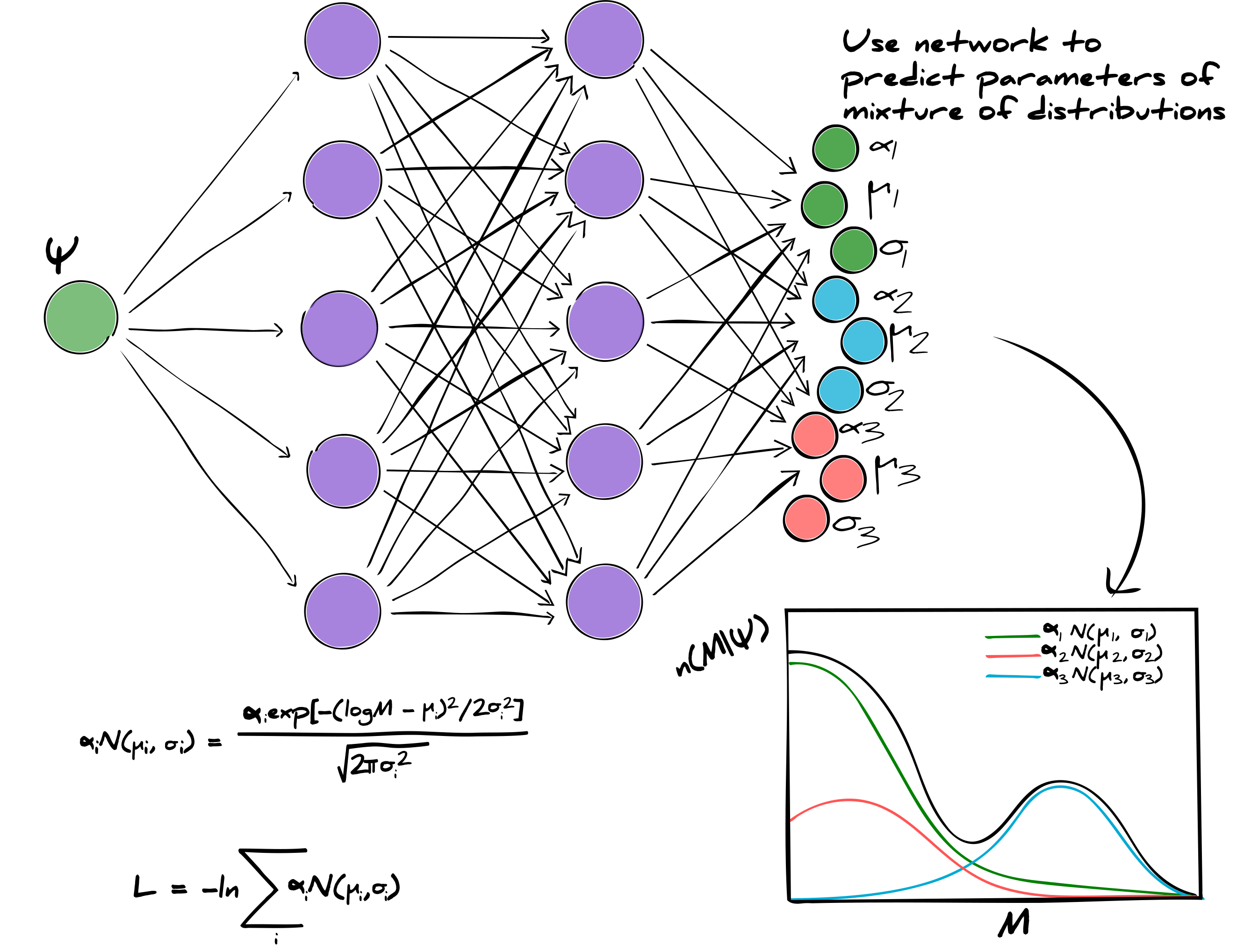
Hey presto - we've got the posterior!
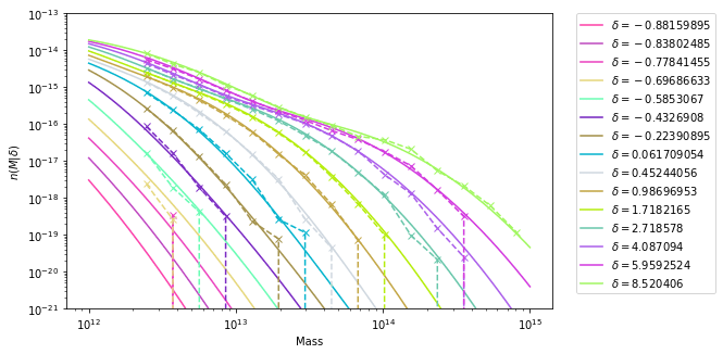
MDNs are not only for probabilities
We can learn generic functions
Autoregressive flows
Improving on MDNs
With MDNs we have to assume a final distribution (mixture of Gaussians, etc.)
We also work only on the posterior distribution (or the likelihood if we work backwards)
Learning the whole probability space
The joint space of data and parameters $\boldsymbol{\psi}=\{{\bf d}, \boldsymbol{\theta}\}$ and networks help learn the true distribution
Normalising flows
A simple way to learn this space is by making a guess for the distribution and then squashing and squeezing it into place.
This can be done using normalising flows $\mathscr{f}:\boldsymbol{\psi}\to\boldsymbol{\chi}$ - a series of invertible transformation of the initial distribution $$\mathscr{f} = \mathscr{f}_0 \odot \mathscr{f}_1 \odot \cdots \odot \mathscr{f}_k$$
The joint distribution (which can be complex and weird) is found using
$$\mathcal{P}(\boldsymbol{\psi}) = \mathcal{P}_\boldsymbol{\chi}(\mathscr{f}^{-1}(\boldsymbol{\psi}))\left|\textrm{det}\frac{\partial\mathscr{f}^{-1}}{\partial\boldsymbol{\psi}}\right|$$where the initial guess $\mathcal{P}_\boldsymbol{\chi}$ can be simple.
We just need to find the transformation $\mathscr{f}$!
Autoregressive models
We can build probability distribution out of conditional probability distributions
$$\mathcal{P}(\boldsymbol{\psi})=\prod_{d=1}^D\mathcal{P}(\psi_d|\psi_{1:d−1})$$Each conditional probability distribution depends on all of the previous inputs from the input vector.
We model the conditionals with simple distributions
A neural network with variable input sizes predicts MDN-like parameters
- The number of inputs defines the conditionality of the distribution of the coniditional distributions
Cosmic shear inference
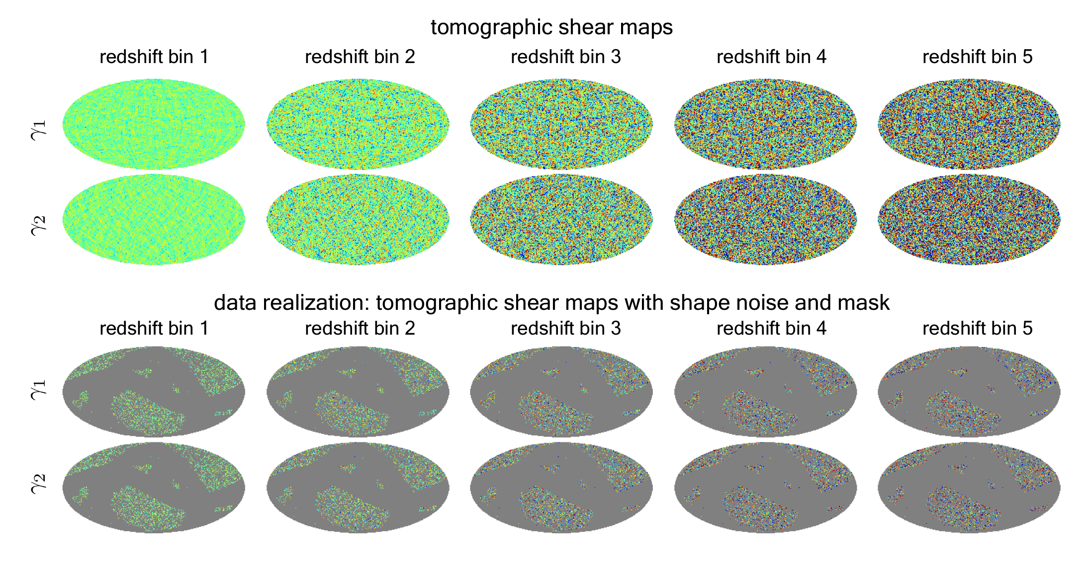
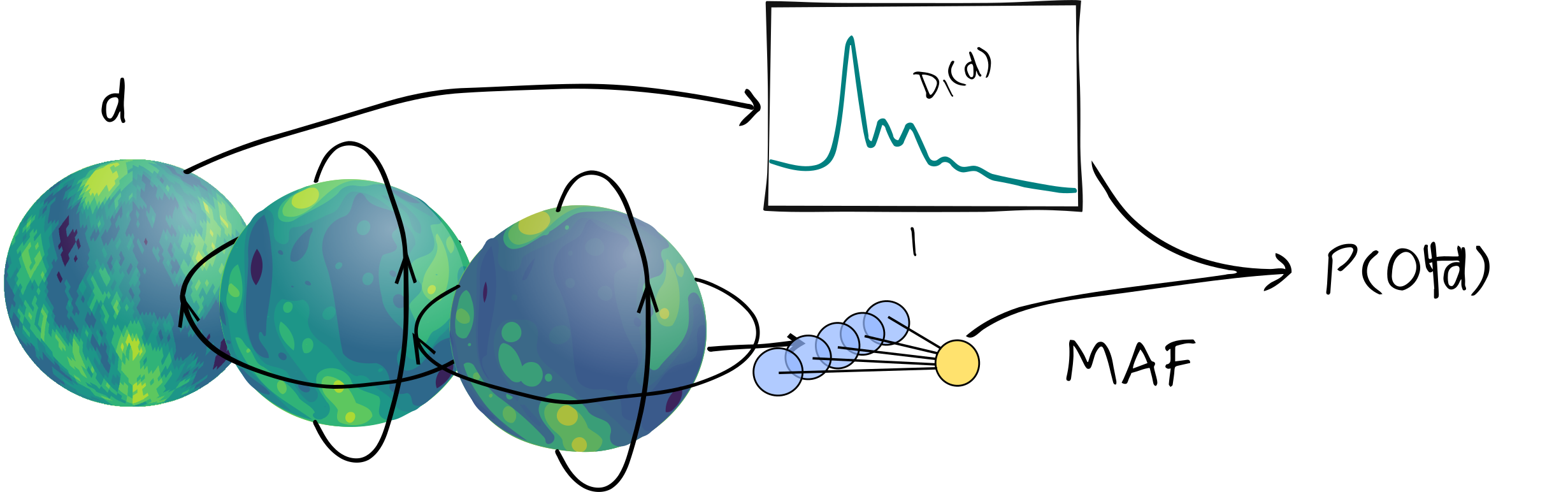
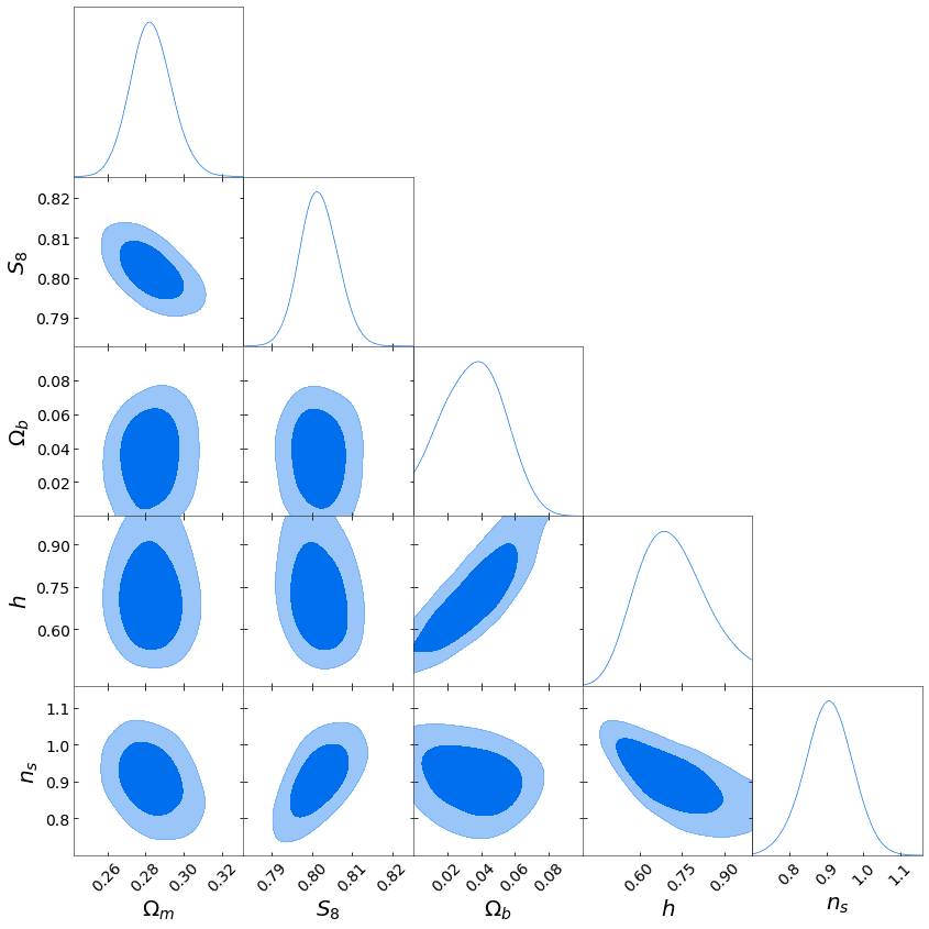
Cosmological parameter constraints
How can we trust our networks?
No networks are impervious to mode collapse
It would be great if we could understand how uncertain we are about our network's outputs.
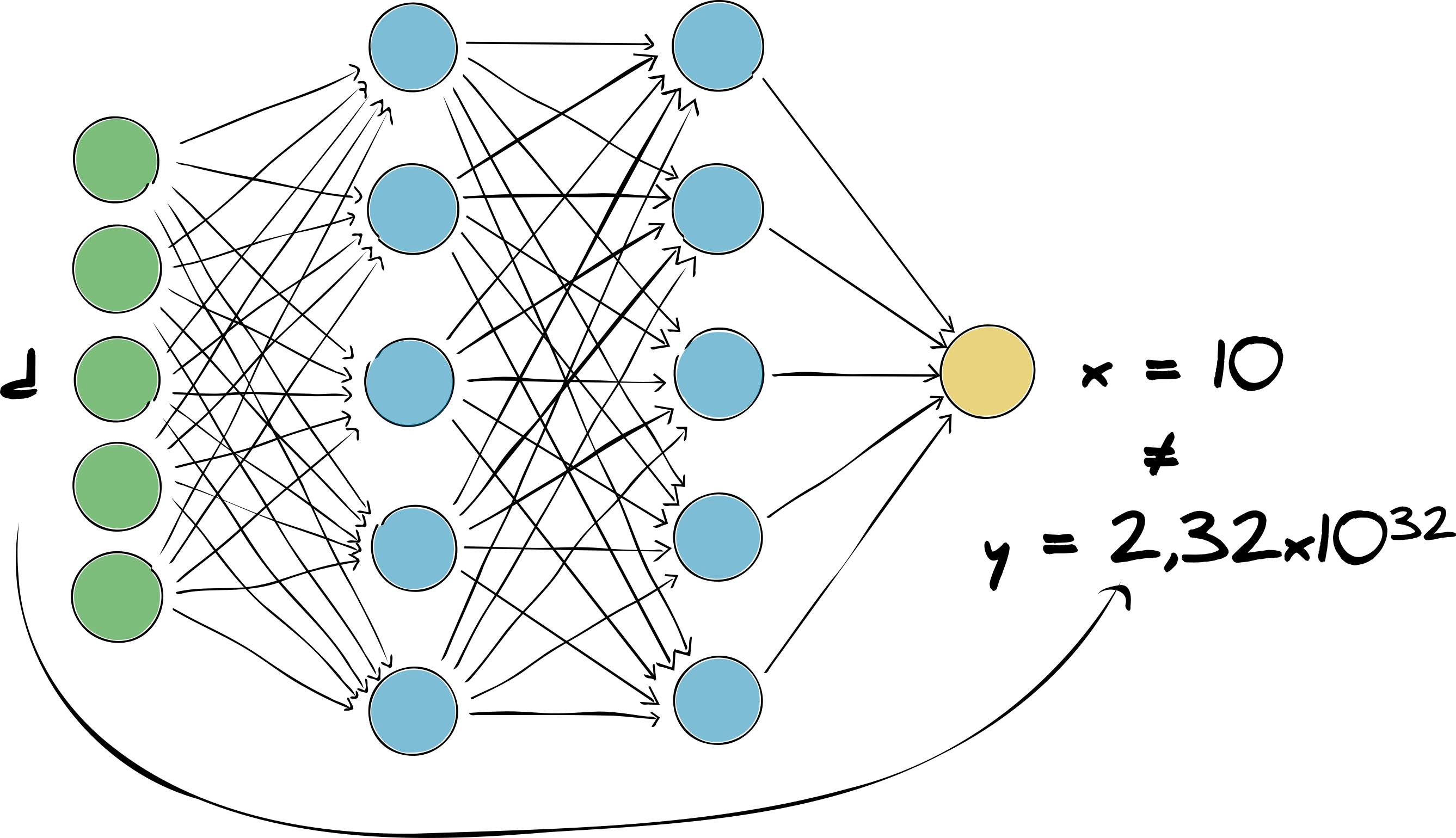
To do so we must think statistically again!
Stats time (again)
A network is just a universal map
$$\mathscr{f}_\boldsymbol{v}:\mathbb{R}^{d}\to \mathbb{R}^{x}$$where an input ${\bf d}$ is mapped to an output ${\bf x}=\mathscr{f}({\bf d}, \boldsymbol{v})$ where $\mathscr{f}$ is tuned via trainable parameters, $\boldsymbol{v}$.
The probability of getting output ${\bf x}$ given some set of network parameters $\boldsymbol{v}$ and input data ${\bf d}$ is described by $\mathcal{L}({\bf x}|\boldsymbol{v},{\bf d})$.
$$\mathcal{P}(\boldsymbol{v}|{\bf x},{\bf d}) = \frac{\mathcal{L}({\bf x}|\boldsymbol{v},{\bf d})p(\boldsymbol{v}|{\bf d})}{p({\bf x}|{\bf d})}$$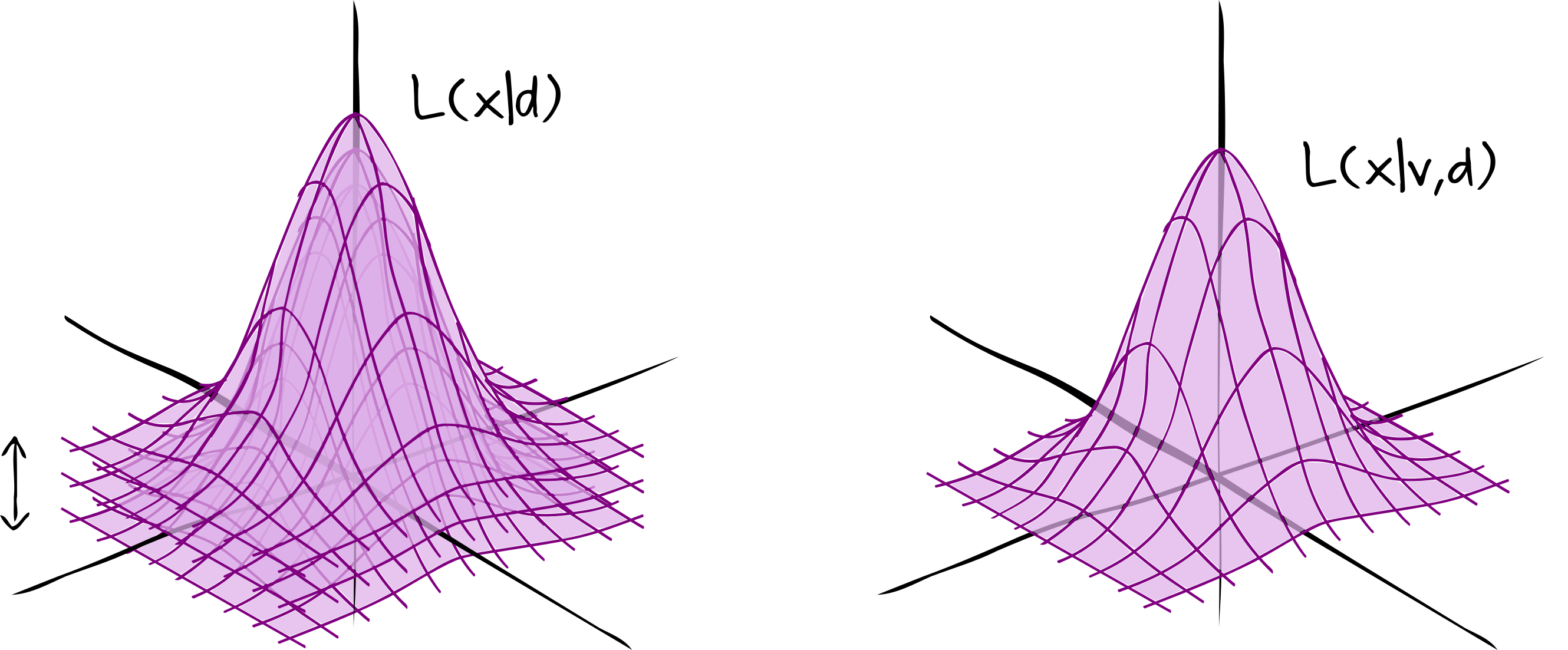
Optimisation is equivalent to maximum likelihood estimation
$$\boldsymbol{v}_\textrm{MLE}=\underset{\boldsymbol{v}\in\boldsymbol{V}}{\textrm{argmin}}\ln\mathcal{L}({\bf x}|\boldsymbol{v},{\bf d})$$
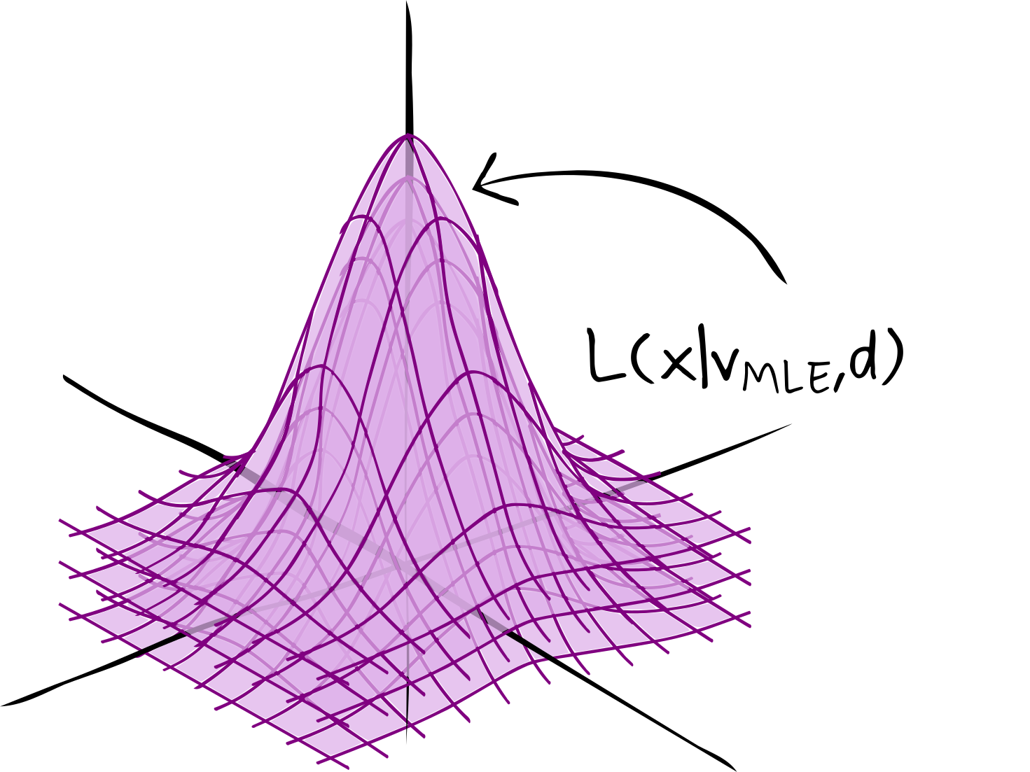
Optimisation with regularisation is equivalent to maximum a posteriori estimation
$$\boldsymbol{v}_\textrm{MAP}=\underset{\boldsymbol{v}\in\boldsymbol{V}}{\textrm{argmin}}\ln\mathcal{L}({\bf x}|\boldsymbol{v},{\bf d})p(\boldsymbol{v}|{\bf d})$$
Unfortunately you can't - but you can try and understand your output in terms of the network parameters
What can we say about the output given our network parameters?
Describe our network parameters via distributions
There are several ways to do this
- Stacked outputs
- Variational Bayes (variational inference)
- Bayesian neural networks (BNN)
- BNN done effectively
Stacked outputs
$$\mathcal{P}({\bf x}|\boldsymbol{v},{\bf d})\approx\textrm{KDE}(\{{\bf x}_n|n\in\textrm{number of NN}\})$$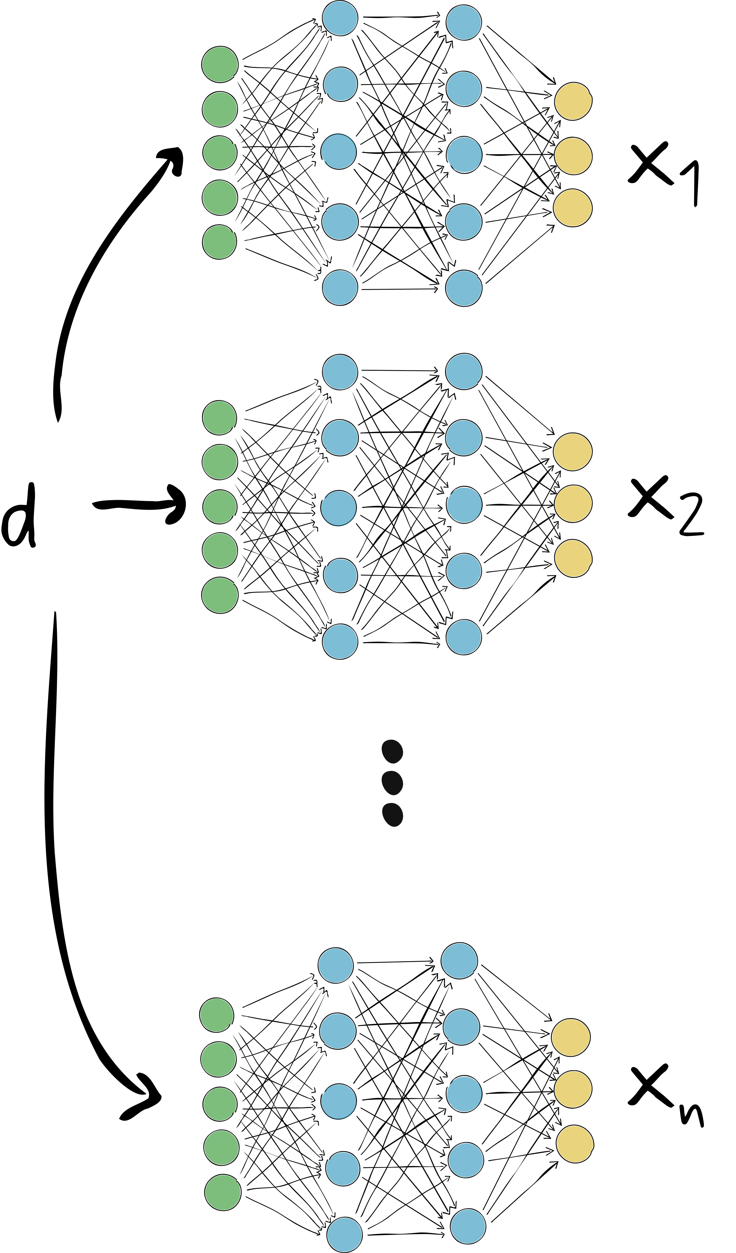
Unfortunately it doesn't really work unless you have LOADS of networks.
(A bit dangerous - but less so than not doing it)
Variational Bayes (inference)
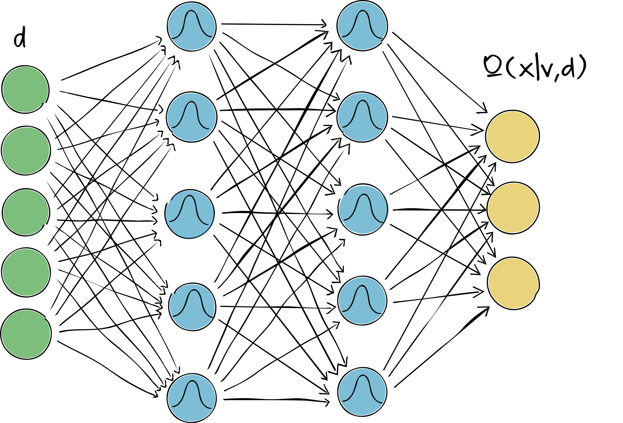
Optimise the network using the KL-divergence (statistical difference measure (measure of the Shannon information)) between $\mathcal{Q}({\bf x}|\boldsymbol{v},{\bf d})$ and the true distribution $\mathcal{P}({\bf x}|\boldsymbol{v},{\bf d})$.
This moves the distributions of the weights around rather than the weights themselves
Really helps with optimisation and gives distributions as outputs!
Very limiting on the form of the final distribution $\mathcal{Q}({\bf x}|\boldsymbol{v},{\bf d})$ which will never really become $\mathcal{P}({\bf x}|\boldsymbol{v},{\bf d})$
Bayesian neural networks
Instead of forcing the form of the weights, we should really sample them
$$\mathcal{P}(\boldsymbol{v}|{\bf x},{\bf d}) \propto \mathcal{L}({\bf x}|\boldsymbol{v},{\bf d})p(\boldsymbol{v}|{\bf d})$$Real outputs are available by marginalising the weights out
Many techniques for sampling, such as Markov chain Monte-Carlo
In practise the number of weights is too high dimensional to do this
Hamiltonian Monte Carlo on network weights
(the proper way)
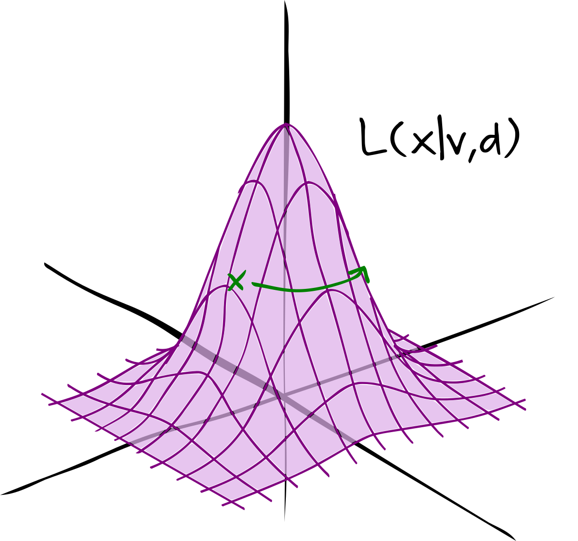
The problem is that you need the gradient of your likelihood with respect to your weights
But that is exactly what you get with a neural network!
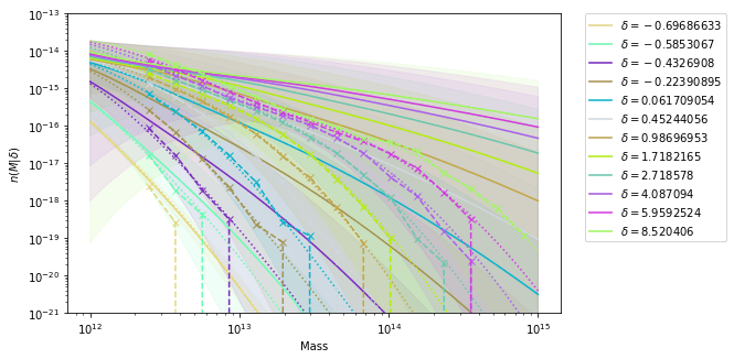
It is possible to sample the weights of your network in high dimensions using HMC!
(it is still quite expensive)
Okay - now relax
Machine learning is fun
It's super useful everywhere - especially in astrophysics
It's a statisticians best friend
You can do loads of cool things
You should never trust it
But you should also find ways to trust it because it's so useful