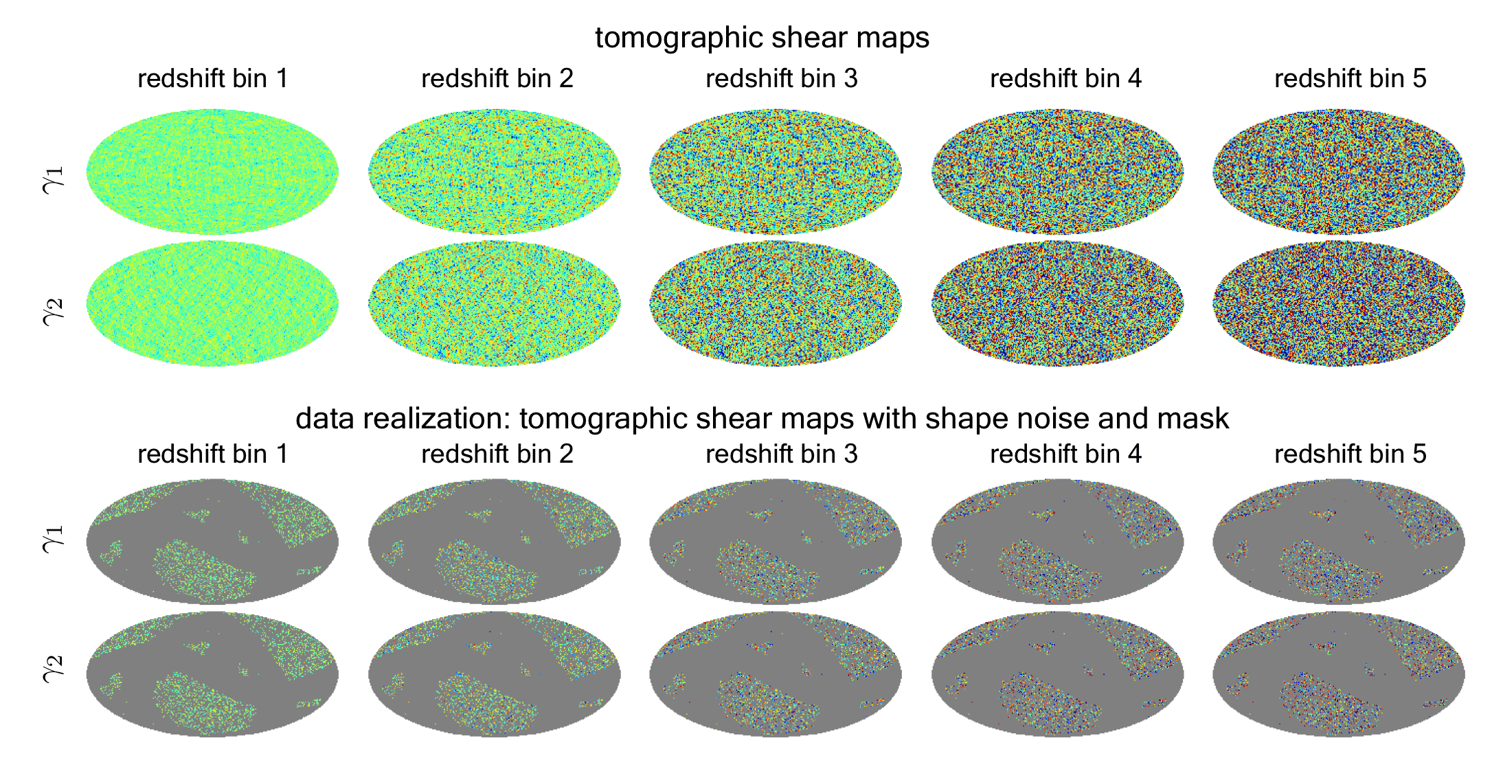
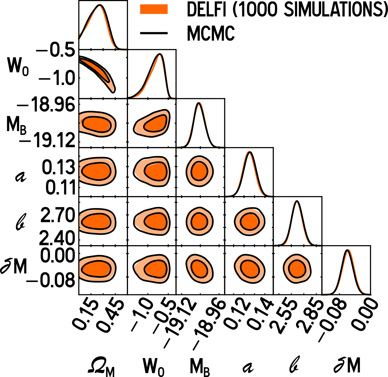
Machine learning for cosmology and Euclid
Tom Charnock
Institut d'Astrophysique de Paris
Slides available at presentations.charnock.fr/ML_Euclid
Play along: git clone https://github.com/tomcharnock/ML_LesHouches.git
or at bit.ly/colab_ML_Euclid








%pylab inline
import jax
import flax
import tqdm
import tensorflow_probability as tfp
import warnings
import os
from scipy.stats import gaussian_kde
warnings.filterwarnings('ignore')
np = jax.numpy
tfp = tfp.experimental.substrates.jax
tfd = tfp.distributions
rng = jax.random.PRNGKey(0)
xkcd();
When we use neural networks we are building statistical models
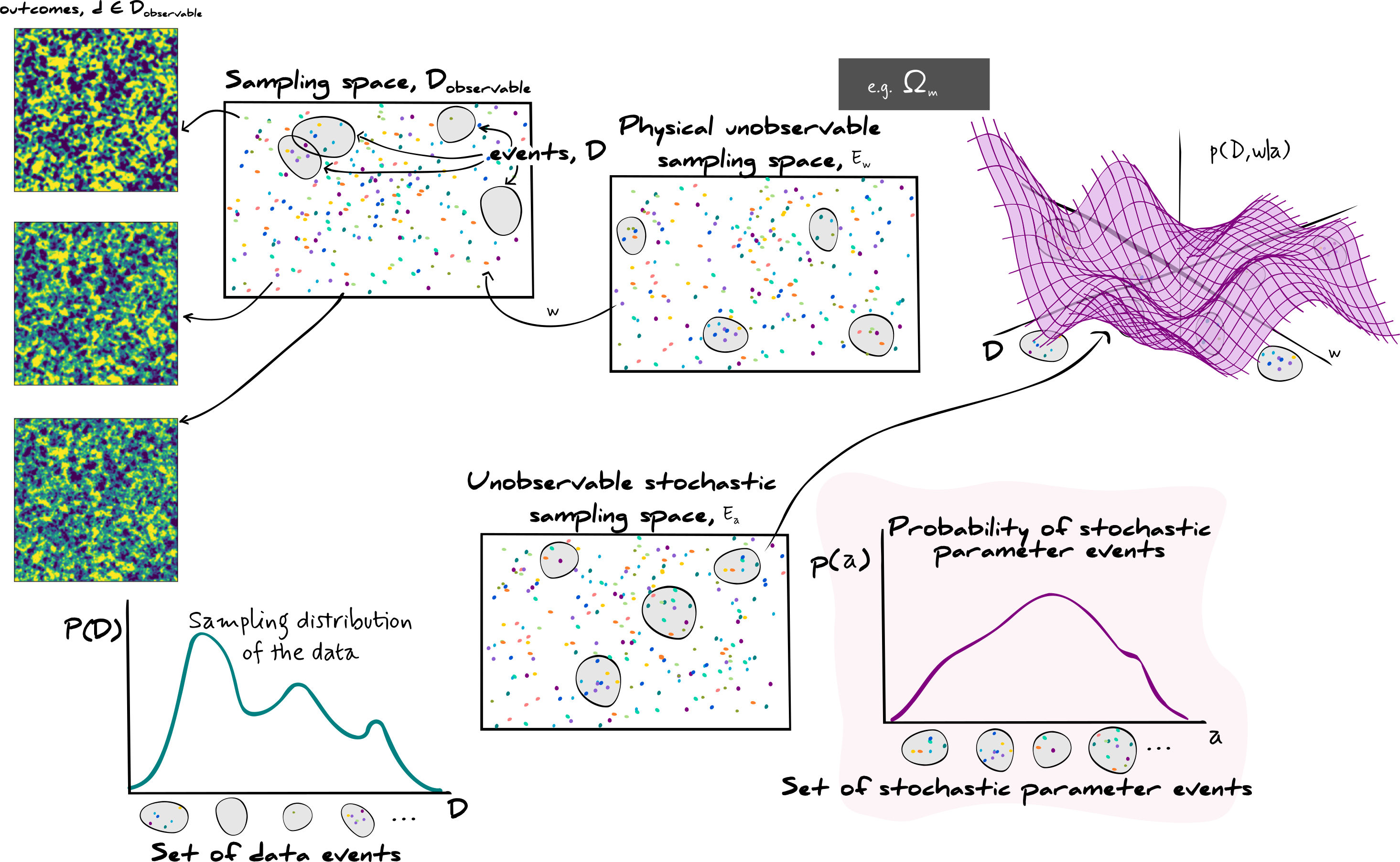
Why do we even care... we should be talking about neural networks!
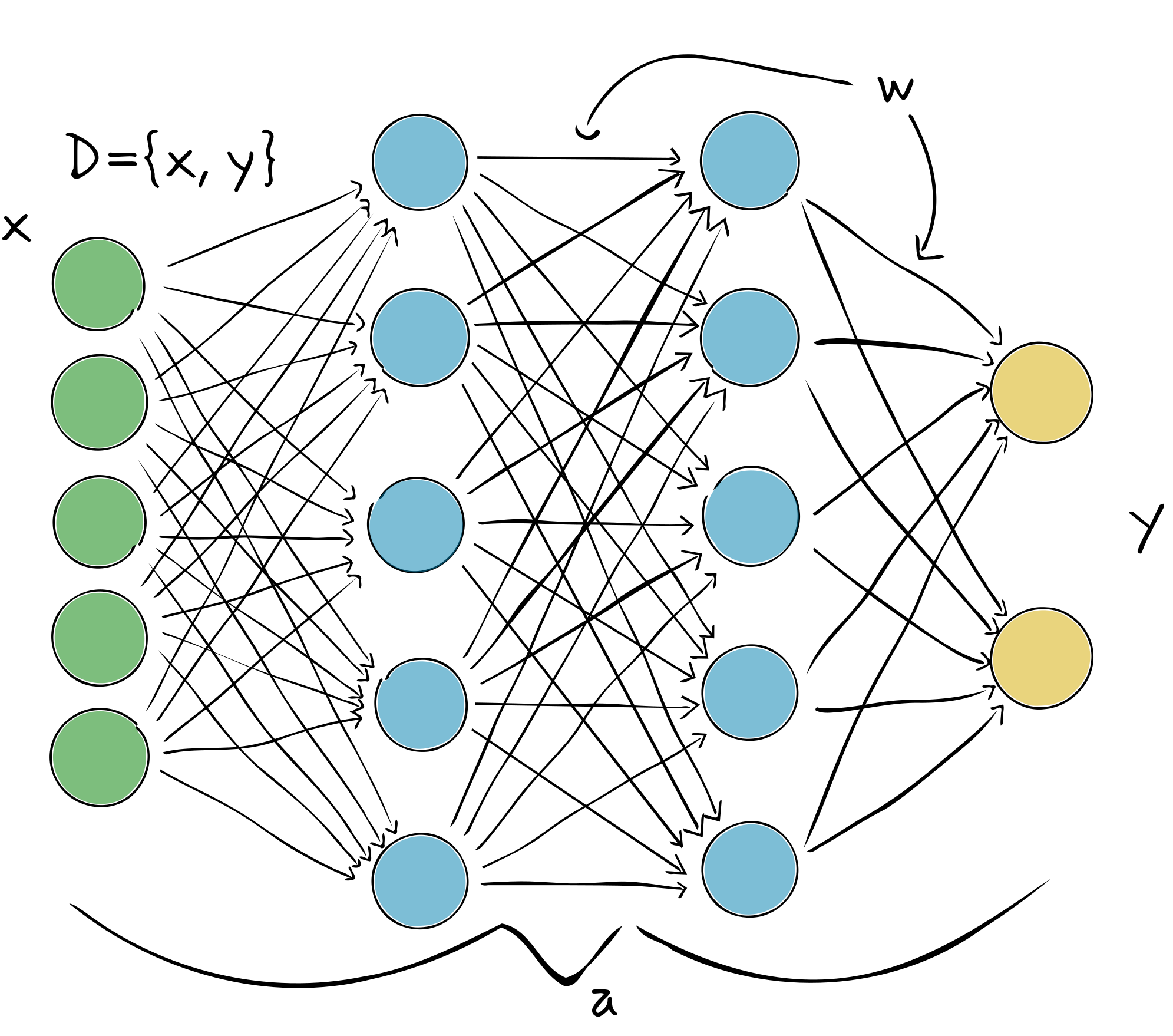
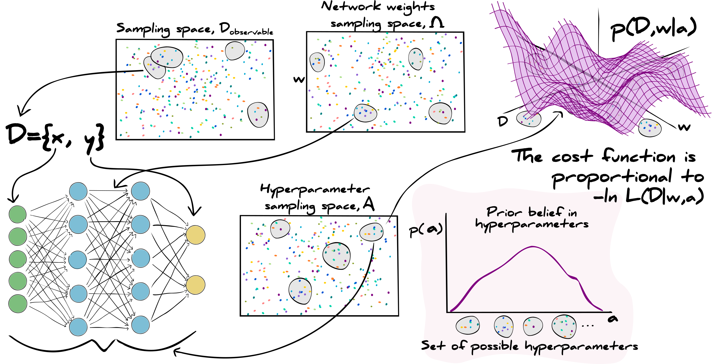
How can we do that?
Variational inference
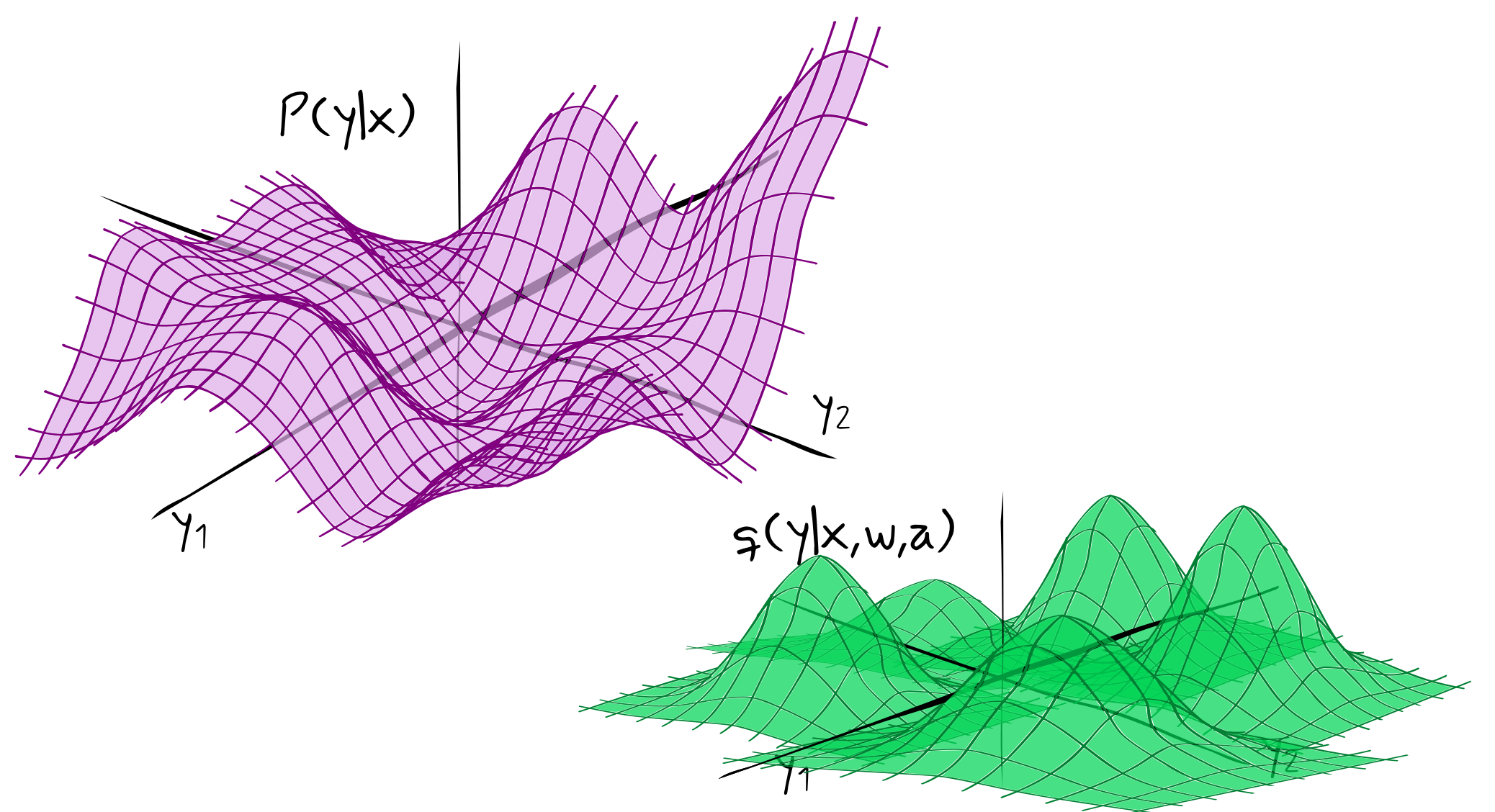
Kullback-Leibler (KL) divergence
A measurement of the information loss by approximating a distribution, $P(y|x)$, with some other distribution, $q(y|x,w,a)$.
$$\mathbb{D}_\textrm{KL}[P(y|x)||q(y|x,w,a)]=\int_{E_y}dyP(y|x)\ln\frac{P(y|x)}{q(y|x,w,a)}$$fig, ax = subplots(1, 1, figsize=(20, 16)); ax_ = ax.twinx(); x_axis=np.linspace(-5, 5, 1000); ax.set_xlim([-5, 5]);ax_.set_ylim([-0.065, 0.45]);ax.set_xlabel("x", fontsize=20);ax_.set_ylabel("Probability density", fontsize=20);ax.set_ylabel("Log density ratio", fontsize=20);ax.tick_params(axis="both", labelsize=20);ax_.tick_params(axis="both", labelsize=20)
ax.fill_between(x_axis, 0, np.log(((tfd.Normal(2, 3).prob(x_axis) + tfd.Normal(-1, 1).prob(x_axis))/2)/tfd.Normal(0, 1).prob(x_axis)), color="C2", alpha=0.5, label="Log ratio")
ax_.plot(x_axis, (tfd.Normal(2, 3).prob(x_axis) + tfd.Normal(-1, 1).prob(x_axis))/2, linewidth=3, label="P(y|x)")
ax_.plot(x_axis, tfd.Normal(0, 1).prob(x_axis), linewidth=3, label="q(y|x,w,a)")
ax_.legend(frameon=False, fontsize=20);

Identical distributions
$$\mathbb{D}_\textrm{KL}[P(y|x)||q(y|x,w,a)]=0\textrm{ means }P(y|x)=q(y|x,w,a)$$Different distributions
$$\mathbb{D}_\textrm{KL}[P(y|x)||q(y|x,w,a)]>0\textrm{ means }P(y|x)\ne q(y|x,w,a)$$Non-symmetric (not a real distance metric)
$$\mathbb{D}_\textrm{KL}[P(y|x)||q(y|x,w,a)]\ne[\mathbb{D}_\textrm{KL}[q(y|x,w,a)||P(y|x)]$$What is the KL-divergence?
$$\begin{align*} \mathbb{D}_\textrm{KL}[P(y|x)||q(y|x,w,a)]&=\int_{E_y}dyP(y|x)\ln\frac{P(y|x)}{q(y|x,w,a)}\\ &=-\int_{E_y}dyP(y|x)\ln q(y|x,w,a)+\int_{E_y}dyP(y|x)\ln P(y|x) \end{align*}$$Entropy of $P(y|x)$
Cross entropy between $P(y|x)$ and $q(y|x,w,a)$
The cross-entropy measures the average number of bits of information needed to tell that an event is drawn from $q(y|x,w,a)$ rather than $P(y|x)$
We don't actually know $P(x,y)$
We might have a sampling distribution, $P(\{x,y\}_\textrm{train})$, made up of
$$\{x_i,y_i\sim P(x,y)|i\in[1,n_\textrm{train}]\}$$(hopefully very close to $\approx P(x,y)$)
Using this sampling distribution we can rewrite the KL divergence as
$$\mathbb{D}_\textrm{KL}[P(y|x)||q(y|x,w,a)]=-\sum_{i=1}^{n_\textrm{train}}P(y_i|x_i)\ln q(y_i|x_i,w,a)+\sum_{i=1}^{n_\textrm{train}}P(y_i|x_i)\ln P(y_i|x_i)$$By minimising the KL-divergence we can attempt to bring $q(y|x,w,a)$ close to $P(y|x)$
(or at least $P(y_\textrm{train}|x_\textrm{train})$).
Entropy term, $P(y|x)$ is independent of $w$, so optimising the parameters of $q(y|x,w,a)$ is equivalent to minimising the cross-entropy
$$\begin{align*} \widehat{w}&=\underset{w\in E_w}{\textrm{arg min}}\,\mathbb{D}_\textrm{KL}[P(y|x)||q(y|x,w,a)]\\ &=\underset{w\in E_w}{\textrm{arg min}}\,-\sum_{i=1}^{n_\textrm{train}}P(y_i|x_i)\ln q(y_i|x_i,w,a) \end{align*}$$How can we calculate the cross entropy?
The likelihood of a training set is
- how often (or the probability, $P(y_\textrm{train}|x_\textrm{train})$, of) each event, $y_i$, in the training set
- the estimation of the probability using the likelihood, $q(y_i|x_i,w,a)$, for every event
Taking the logarithm (divided by the number of training samples) gives
$$\begin{align*} \frac{1}{n_\textrm{train}}\ln L(y_\textrm{train}|x_\textrm{train})&=\frac{1}{n_\textrm{train}}\ln\prod_{i=1}^{n_\textrm{train}}q(y_i|x_i,w,a)^{n_\textrm{train}P(y_i|x_i)}\\ &=\sum_{i=1}^{n_\textrm{train}}P(y_i|x_i)q(y_i|x_i,w,a) \end{align*}$$Minimising the cross-entropy is equivalent to maximising the logarithm of the likelihood!
Maximum-likelihood estimation!
$$\widehat{w}=\underset{w\in E_w}{\textrm{arg min}}-\ln L(y_\textrm{train}|x_\textrm{train})$$
Equivalent to minimising the KL-divergence and bringing $q(y|x,w,a)$ as close to $P(y|x)$ as possible
False
Neural networks only predict parameters, $Y=f_{w,a}(x)$, of a distribution that we choose.
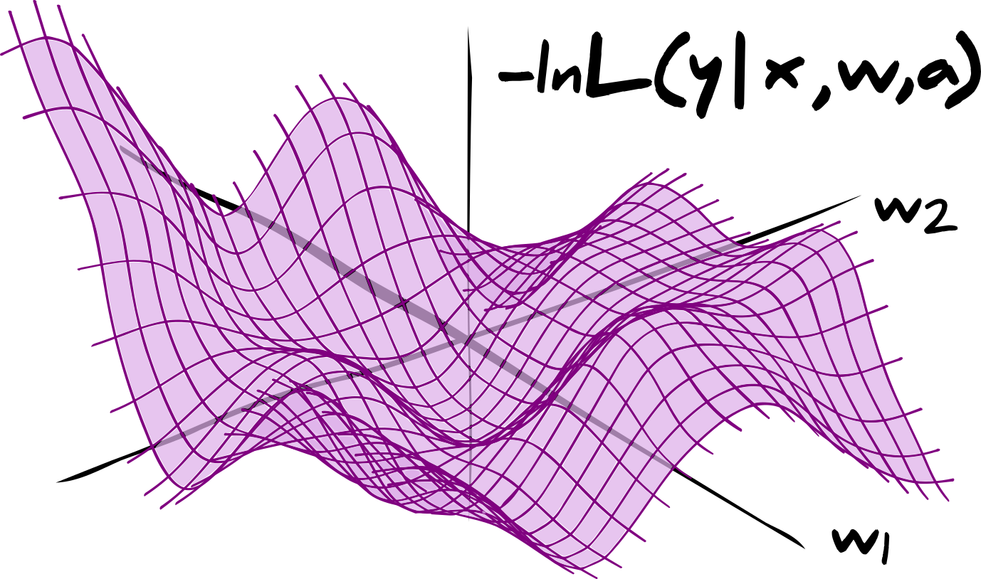
The $Y$ should not be interpreted as predictions of $y$ from $(x, y)$
Example time!
n_train_sims = 1000; x = np.linspace(0, 10, 100).astype(np.float32)
def simulator(m, key):
return (m * x[np.newaxis, :] + jax.random.normal(key, shape=(m.shape[0],) + x.shape))
rng, key = jax.random.split(rng)
m = jax.random.uniform(key, minval=-5, maxval=5, shape=(n_train_sims, 1))
rng, key = jax.random.split(rng)
y = simulator(m, key)
split = 0.1
m_train = m[:int(n_train_sims * (1 - split))]
y_train = y[:int(n_train_sims * (1 - split))]
m_validate = m[int(n_train_sims * (1 - split)):]
y_validate = y[int(n_train_sims * (1 - split)):]
figure("Training data", figsize=(20, 16)); xlabel("x", fontsize=20); xlim([0, 10]); ylabel("y train", fontsize=20);tick_params(axis="both", labelsize=20)
plot(x, y_train.T[:, ::10], alpha=0.6);

Now lets make a neural network to estimate $m$.
We're going to make two identical networks
- train traditionally
- explicitly characterise a probabilistic model, $L(m|y,w,a)=\mathbb{N}\left(f_{w,a}(y),\mathbb{I}\right)$
@flax.nn.module
def dense_predictor(x):
x = flax.nn.Dense(x, 128)
x = flax.nn.leaky_relu(x, 0.01)
x = flax.nn.Dense(x, 128)
x = flax.nn.leaky_relu(x, 0.01)
x = flax.nn.Dense(x, 1)
return x
rng, key = jax.random.split(rng)
_, initial_params = dense_predictor.init_by_shape(
key, [((100,), np.float64)])
mse_model = flax.nn.Model(dense_predictor, initial_params)
mse_opt = flax.optim.Adam(1e-5).create(mse_model)
tfp_model = flax.nn.Model(dense_predictor, initial_params)
tfp_opt = flax.optim.Adam(7e-6).create(tfp_model)
So classically we might want to regress to the esimate using mean squared error as a loss function $$\Lambda = \frac{1}{N}\sum_{i=1}^N(f_{w,a}(y_i)-m_i)^2$$
@jax.jit
def mse(y, m, model):
def fn(y, m):
return np.mean((model(y) - m)**2.)
return np.mean(jax.vmap(fn)(y, m))
Lets also maximise the log likelihood, i.e. minimise the cross entropy, i.e.i.e minimise the KL divergence
@jax.jit
def negloglike(y, m, model):
def fn(y, m):
return np.mean(-tfd.Normal(loc=model(y), scale=1).log_prob(m))
return np.mean(jax.vmap(fn)(y, m))
Now we do the optimisation of the weights via backpropagation
$$\begin{align*} w_i&\leftarrow w_i+\eta\partial_{w_i}\textrm{MSE}(f_{w,a}(y_\textrm{train}), m_\textrm{train})\\ w_i&\leftarrow w_i+\eta\partial_{w_i}-\ln\mathbb{N}(f_{w,a}(y_\textrm{train}), \mathbb{I}|m_\textrm{train}) \end{align*}$$(Actually we're going to use Adam, but you get the idea)
@jax.jit
def optimise(mse_opt, tfp_opt):
def get_mse(model):
return mse(y_train, m_train, model)
def get_negloglike(model):
return negloglike(y_train, m_train, model)
mse_loss, mse_grad = jax.value_and_grad(get_mse)(mse_opt.target)
negloglike_loss, negloglike_grad = jax.value_and_grad(get_negloglike)(tfp_opt.target)
mse_opt = mse_opt.apply_gradient(mse_grad)
tfp_opt = tfp_opt.apply_gradient(negloglike_grad)
return mse_opt, tfp_opt, [mse_loss, negloglike_loss]
And fit the models (for 1000 epochs) (we'll also validate the network with our unseen validation set to evaluate the performance)
epochs = 1000; loss = []; val_loss = []; bar = tqdm.tnrange(epochs, desc="iterations")
for i in bar:
mse_opt, tfp_opt, loss_ = optimise(mse_opt, tfp_opt)
loss.append(loss_)
val_loss.append([
mse(y_validate, m_validate, mse_opt.target),
negloglike(y_validate, m_validate, tfp_opt.target)])
bar.set_postfix(loss=loss[i], val_loss=val_loss[i])
loss = np.array(loss); val_loss = np.array(val_loss)
fig, ax1 = subplots(figsize=(20, 16)); ax2 = ax1.twinx(); epo1 = np.arange(1, epochs+1); labels = ["MSE (train)", "-log L(m|y train)", "MSE (validation)", "-log L(m|y validate)"]; ax1.set_xlim([1, epochs]); ax1.set_xlabel("Epochs", fontsize=20); ax1.set_ylabel("MSE", fontsize=20); ax2.set_ylabel("-log P(m|y)", fontsize=20); ax1.tick_params(axis="both", labelsize=20); ax2.tick_params(axis="both", labelsize=20); fig.suptitle="Training iterations"
a = ax1.loglog(epo1, loss[:, 0], linewidth=3)
b = ax2.loglog(epo1, loss[:, 1], linestyle="dashed", linewidth=3)
c = ax1.loglog(epo1, val_loss[:, 0], linewidth=3)
d = ax2.loglog(epo1, val_loss[:, 1], linestyle="dashed", linewidth=3)
legend(a+b+c+d, labels, fontsize=20);

n_test_sims = 100
rng, key = jax.random.split(rng)
m_test = jax.random.uniform(key, minval=-5, maxval=5, shape=(n_test_sims, 1))
rng, key = jax.random.split(rng)
y_test = simulator(m_test, key)
m_predicted = mse_opt.target(y_test)
m_estimated_mean = tfd.Normal(tfp_opt.target(y_test), scale=1).mean()
figure("Predicted m", figsize=(20, 16)); plot([-5, 5], [-5, 5], linestyle="dashed", color="black",linewidth=3); xlabel("m predicted", fontsize=20); xlim([-5, 5]); ylabel("m test", fontsize=20); ylim([-5, 5]); tick_params(axis="both", labelsize=20)
scatter(m_predicted, m_test, color="C0", s=250, label="MSE")
scatter(m_estimated_mean, m_test, color="C1", marker="+", s=250, label="log P(m|y)")
legend(fontsize=20);

So network outputs are just the parameters of a probabilistic model that we choose as a description of our problem
Using the MSE is equivalent to saying that you believe the distribution, $P(y|x)$, is able to be modelled as a Gaussian with locations given by the network output.
(whether or not this is a good choice is a different question)
Note that the same is true for minimising the binary cross-entropy
- Equivalent to fitting the parameters of a Bernoulli distribution to minimise the KL divergence, $P(y|x)\approx q(y|x,w,a)=\textrm{Bernoulli}(f_{w,a}(x))$
And minimising absolute error
- Equivalent to fitting the parameters of a Laplacian distribution to minimise the KL diverenge, $P(y|x)\approx q(y|x,w,a)=\textrm{Laplacian}(f_{w,a}(x))$
Training a neural network is doing variational inference
Since we have made a stochastic model, $q(y|x,\widehat{w},a)$, of $P(y|x)$ we get estimated uncertainties of $y$ for free
figure("Probabilistic model for m", figsize=(20, 16)); plot([-5, 5], [-5, 5], color="black", linestyle="dashed", linewidth=3); xlim([-4, 4]); xlabel("m predicted", fontsize=20); ylim([-4, 4]); ylabel("m test", fontsize=20); tick_params(axis="both", labelsize=20); m_eval = np.linspace(-5, 5, 100).reshape(1, 1, -1);
contourf(m_eval[0, 0], m_test[:, 0], tfd.Normal(tfp_opt.target(y_test), scale=1).prob(m_eval)[0], levels=50)
cbar = colorbar(); cbar.set_label("P(m|y)", fontsize=20); cbar.ax.tick_params(labelsize=20)
scatter(tfd.Normal(tfp_opt.target(y_test), scale=1).mean(), m_test[:, 0], s=100);

Note this doesn't tell us if our estimate is actually any good.
- Specifically, because we only calculate the cross entropy, we ignore the entropy in the minimisation of the KL-divergence, whose calculation would actually tell us whether the distributions were identical.
- Note that this is only true for the sampling distribution of data that we have and not the true distribution of all possible data. We might look a bit more into this tomorrow.
Generating data
Cosmological and astrophysical data from galaxy surveys is very complex
Hard (or expensive) to model
Impossible to write down the likelihood
Can we generate this data more efficiently using machine learning?
Generative models
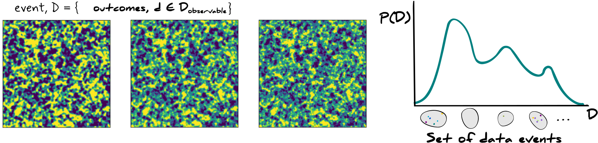
How can we generate samples $D\sim P(D)$ cheaply?
- We have some training set $\{D_i\sim P(D)|i\in[0, n_\textrm{train}]\}$
- We know we can model distributions using NN (in fact, that is their only purpose 😉)
Latent variables
A latent variable is a random variable from some distribution, $z\sim P(z)$
We can describe the probability of any data AND latent parameter as $P(D,z)$.
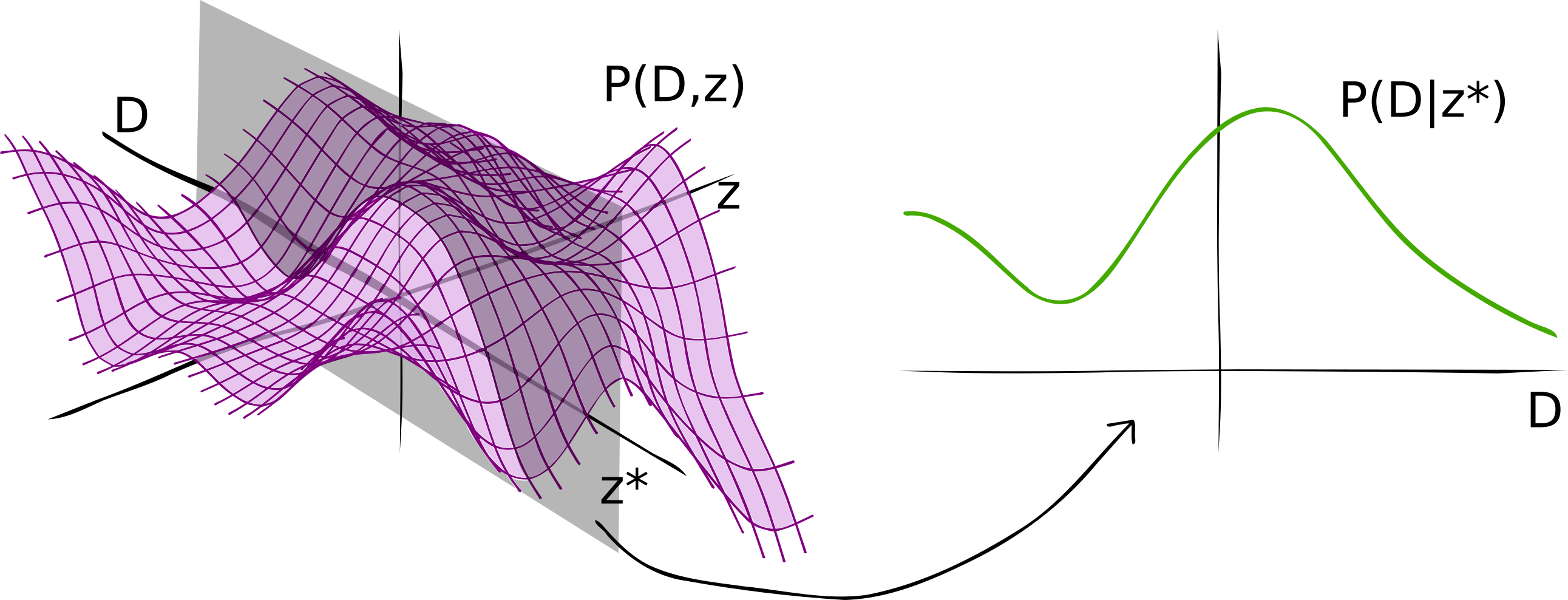
The distribution of data can be obtained by marginalising out the latent parameters $$\begin{align*} P(D)&=\int_{E_z}dz\,P(D,z)\\ &=\int_{E_z}dz\,P(D|z)P(z) \end{align*}$$
Why does this help?
We don't know $P(D|z)$ nor $P(z)$
- we can use Bayes theorem to estimate $\displaystyle P(z|D_\textrm{train})=\frac{P(D_\textrm{train}|z)P(z)}{P(D_\textrm{train})}$
Forward and reverse KL-divergence
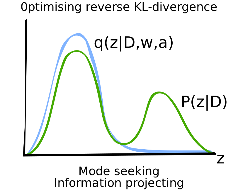
Because we do not know how to take the expectation value with respect to $P(z|D)$ we cannot use the forward KL-divergence
$$\mathbb{D}_\textrm{KL}[P(z|D)||q(z|D,w^e,a^e)]=\int_{E_z}dz\,P(z|D)\ln\frac{P(z|D)}{q(z|D,w^e,a^e)}$$Instead we use reverse KL-divergence
$$\mathbb{D}_\textrm{KL}[q(z|D,w^e,a^e)||P(z|D)]=\int_{E_z}dz\,q(z|D,w^e,a^e)\ln\frac{q(z|D,w^e,a^e)}{P(z|D)}$$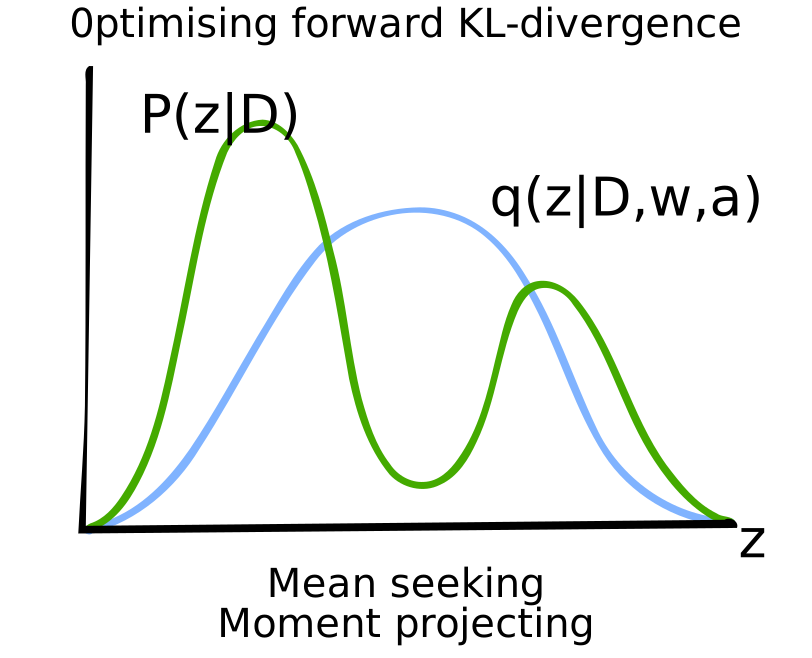
Dealing with the unknown distribution, $P(z|D)$
$$\begin{align*} &\mathbb{D}_\textrm{KL}[q(z|D,w^e,a^e)||P(z|D)]\\ &\phantom{one}=\int_{E_z}dz\,q(z|D,w^e,a^e)\ln\frac{q(z|D,w^e,a^e)}{P(z|D)}\\ &\phantom{one}=\int_{E_z}dz\,q(z|D,w^e,a^e)\ln q(z|D,w^e,a^e)-\int_{E_z}dz\,q(z|D,w^e,a^e)\ln P(z|D)\\ &\phantom{one}=\int_{E_z}dz\,q(z|D,w^e,a^e)\ln q(z|D,w^e,a^e)-\int_{E_z}dz\,q(z|D,w^e,a^e)\ln P(D|z)\\ &\phantom{hello}-\int_{E_z}dz\,q(z|D,w^e,a^e)\ln P(z)+\int_{E_z}dz\,q(z|D,w^e,a^e)\ln P(D)\\ &\phantom{one}=\mathbb{D}_\textrm{KL}[q(z|D,w^e,a^e)||P(z)]-\int_{E_z}dz\,q(z|D,w^e,a^e)\ln P(D|z)+\ln P(D) \end{align*}$$Infamous ELBO
Reorganising the terms gives us $$ \begin{align*}\ln P(D)&=\mathbb{D}_\textrm{KL}[q(z|D,w^e,a^e)||P(z|D)]+\int_{E_z}dz\,q(z|D,w^e,a^e)\ln P(D|z)-\mathbb{D}_\textrm{KL}[q(z|D,w^e,a^e)||P(z)]\\ &=\mathbb{D}_\textrm{KL}[q(z|D,w^e,a^e)||P(z|D)]+\textrm{ELBO}(q(z|D,w,a)) \end{align*}$$
Since $\mathbb{D}_\textrm{KL}[q(z|D,w^e,a^e)||P(z|D)]\ge0$ then we can see that
$$\ln P(D)\ge\textrm{ELBO}(q(z|D,w,a))$$The ELBO is the evidence lower bound!
Maximising the ELBO with respect to $w$ maximises the lower bound on the evidence of the data, and since this evidence is independent of $w$ then this objective minimises the KL divergence between $q(z|D,w,a))$ and $P(z|D)$.
How do we maximise the ELBO?
$$\textrm{ELBO}(q(z|D,w,a))=\int_{E_z}dz\,q(z|D,w^e,a^e)\ln P(D|z)-\mathbb{D}_\textrm{KL}[q(z|D,w^e,a^e)||P(z)]$$Focus on the second term. The reverse KL-divergence with respect to $P(z)$.
What is $P(z)$?
We can assume any distribution that we want for the true distribution of latent parameters - they're latent.
- We normally choose a normal distribution because it's easy, $P(z)=\mathbb{N}({\bf 0}|\mathbb{I})$.
(Side-note) Neural density estimators
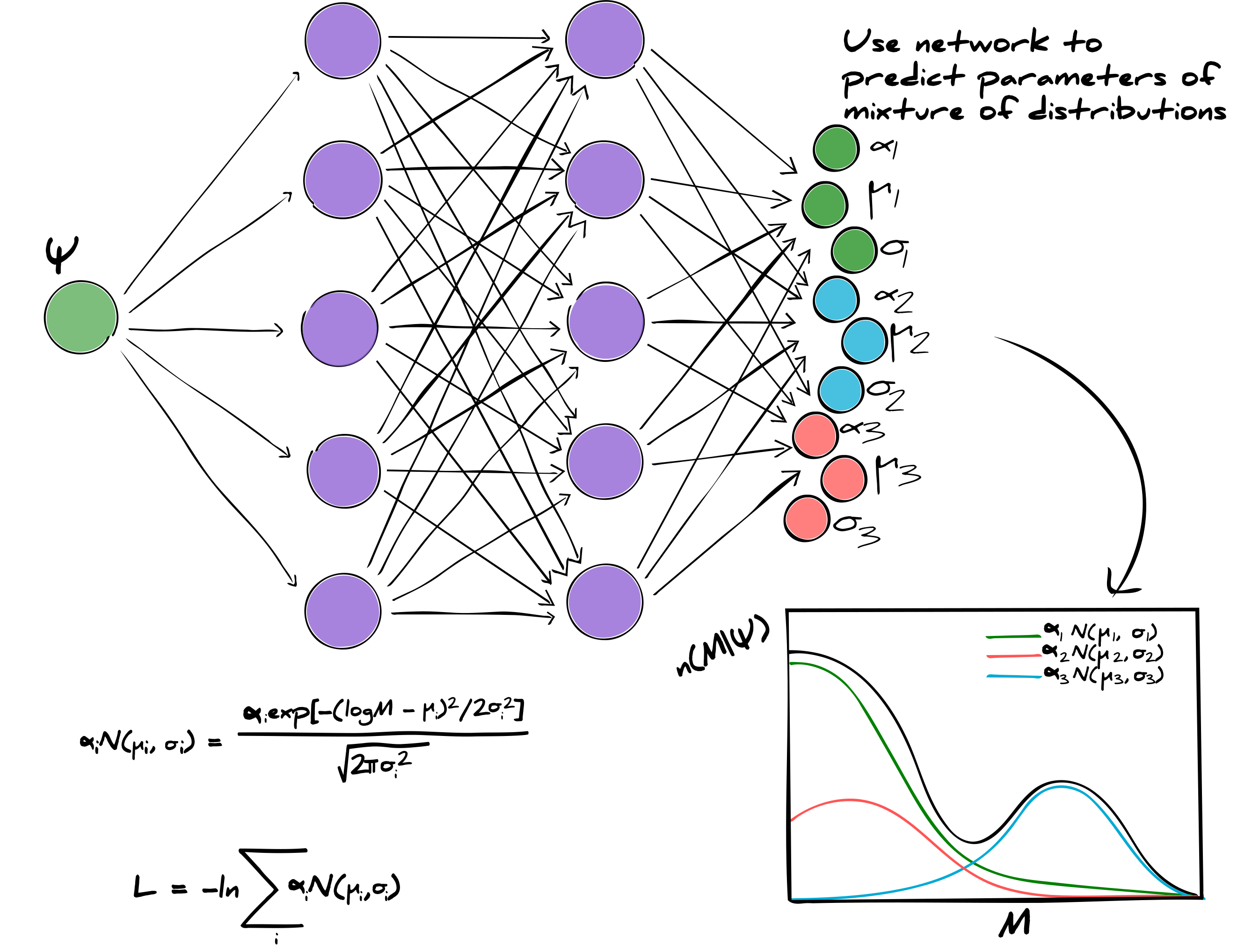
We can write an analytic formula for the KL-divergence
$$\begin{align*} \mathbb{D}_\textrm{KL}[q(z|D,w^e,a^e)||P(z)]&=\int_{E_z}dz\,q(z|D,w^e,a^e)\ln\frac{q(z|D,w^e,a^e)}{P(z)}\\ &=\int_{E_z}dz\,\mathbb{N}(f_{w_\mu^e,a_\mu^e}(D),f_{w_\Sigma^e,a_\Sigma^e}(D))\ln\frac{\mathbb{N}(f_{w_\mu^e,a_\mu^e}(D),f_{w_\Sigma^e,a_\Sigma^e}(D))}{\mathbb{N}({\bf 0},\mathbb{I})}\\ &=\frac{1}{2}\sum_{i=1}^{\textrm{dim }z}\left(\exp[f_{w_\Sigma^e,a_\Sigma^e}(D)]_i+f_{w_\mu^e,a_\mu^e}(D)_i^2-1-f_{w_\Sigma^e,a_\Sigma^e}(D)_i\right) \end{align*}$$First term in the ELBO $$\int_{E_z}dz\,q(z|D,w^e,a^e)\ln P(D|z)$$
We actually want to model the distribution of data $P(D)$ and so we go back to the forward KL-divergence between a variational distribution for $P(D|z)$, i.e. $q(D|z,w^d,a^d)$
$$\int_{E_z}dz\,q(z|D,w^e,a^e)\ln P(D|z)\approx\int_{E_z}dz\,q(z|D,w^e,a^e)\ln q(D|z,w^d,a^d)$$So as before we can minimise the forward KL-divergence (cross-entropy) which is maximising the log likelihood
$$\begin{align*} \widehat{w}^d&=\underset{w^d\in E_{w^d}}{\textrm{arg min}}\,\mathbb{D}_\textrm{KL}[P(D)||q(D|z,w^d,a^d)]\\ &=\underset{w^d\in E_{w^d}}{\textrm{arg min}}\,-\ln L(D_\textrm{train}) \end{align*}$$Wow - this is super complicated... how can we actually do this?
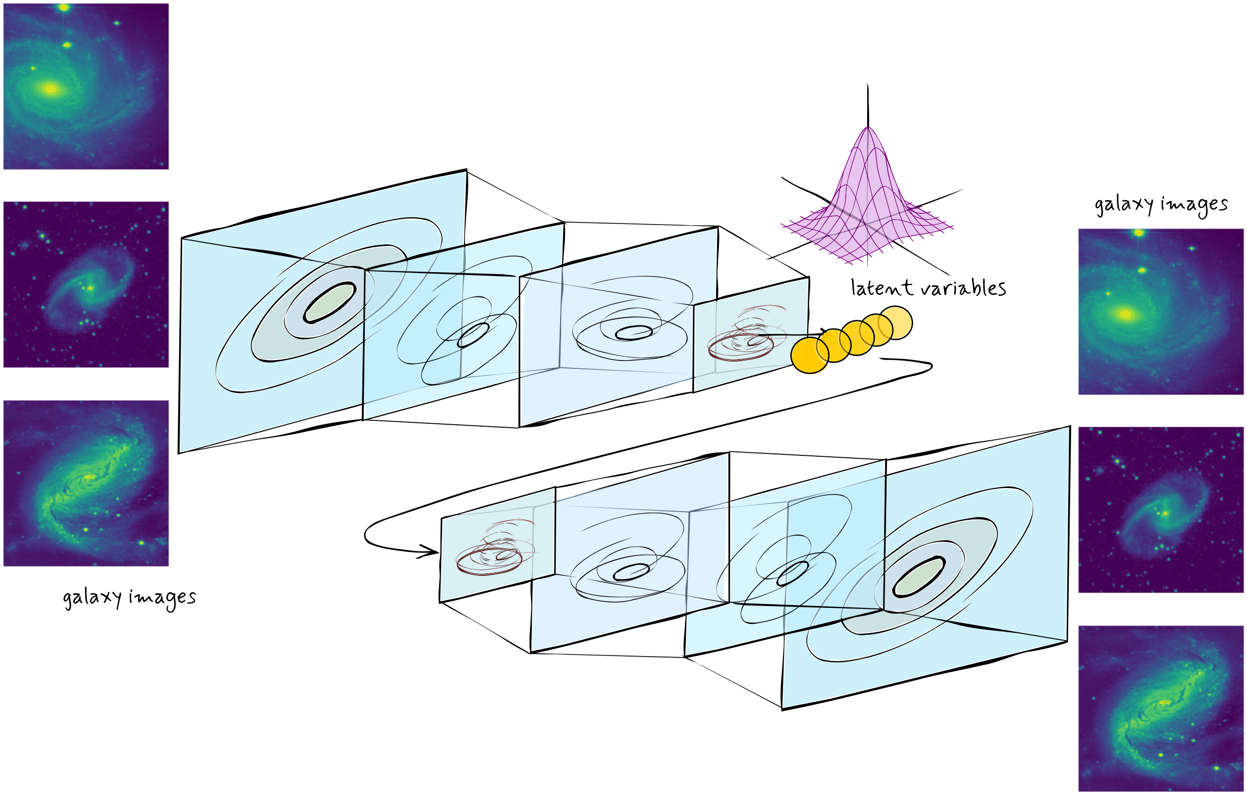
class vae(flax.nn.Module):
def apply(self, D, samples=None, key=None):
loc, scale = self.encoder(D)
N = tfd.Normal(loc, scale)
if (samples is None) or (key is None):
z = np.repeat(N.mean(), 100, axis=-1)
else:
if samples is None:
samples = 1
z = N.sample((samples, 100), seed=key)[..., 0]
if len(z.shape) == 3:
z = np.moveaxis(z, 2, 0)
return self.decoder(z), loc, scale
def encoder(self, x):
x = flax.nn.Dense(x, 32, kernel_init=jax.nn.initializers.normal(1e-6))
x = flax.nn.leaky_relu(x, 0.01)
x = flax.nn.Dense(x, 8, kernel_init=jax.nn.initializers.normal(1e-6))
x = flax.nn.leaky_relu(x, 0.01)
x = flax.nn.Dense(x, 2, kernel_init=jax.nn.initializers.normal(1e-6))
return x[..., ::2], np.exp(x[..., 1::2])
def decoder(self, x):
x = flax.nn.Dense(x, 100, kernel_init=jax.nn.initializers.normal(1e-6))
x = flax.nn.leaky_relu(x, 0.01)
return flax.nn.Dense(x, 100, kernel_init=jax.nn.initializers.normal(1e-6))
We can initialise the neural network and taking a random example of the data we used before see how well the network generates similar data
rng, tfp_key = jax.random.split(rng)
rng, key = jax.random.split(rng)
_, initial_params = vae.init_by_shape(
key, [((100,), np.float32)],
samples=np.int32(1),
key=tfp_key)
vae_model = flax.nn.Model(vae, initial_params)
vae_opt = flax.optim.Adam(1e-3).create(vae_model)
rng, key = jax.random.split(rng)
y_mean, _, _ = vae_model(y_test[3])
y_gen, _, _ = vae_model(y_test[3], samples=10, key=key)
figure("Untrained generated samples", figsize=(20, 16)); xlabel("x", fontsize=20); xlim([0.1, 10]); ylabel("y", fontsize=20);tick_params(axis="both", labelsize=20)
plot(x, y_gen.T, linestyle="dotted", linewidth=3)
plot(x, y_mean, color="black", label="Mean generated sample", linewidth=3)
plot(x, y_test[3], label="Target sample", linewidth=3)
legend(fontsize=20);

@jax.jit
def KL(loc, log_scale):
return np.mean(0.5 * (np.exp(log_scale) + loc**2. - 1. - log_scale), -1)
@jax.jit
def vae_like(y, y_pred):
def fn(y, y_pred):
return np.mean(np.sum(-tfd.Normal(y_pred, scale=1).log_prob(y), -1))
return jax.vmap(fn, in_axes=0)(y, y_pred)
def vae_loss(y, model, key, samples=10):
def run_model(y):
return model(y, samples=samples, key=key)
def get_loss(y_pred, loc, log_scale):
return np.mean(vae_like(y, y_pred) - KL(loc, log_scale))
y_pred, loc, log_scale = jax.jit(run_model)(y)
return jax.jit(get_loss)(y_pred, loc, log_scale)
def vae_optimise(vae_opt, key, samples=10):
def get_vae_grad(model):
return vae_loss(y_train, model, key=key, samples=samples)
def get_vae_grad_jit(model):
return jax.grad(get_vae_grad)(model)
def apply_gradient_jit(grad):
return vae_opt.apply_gradient(grad)
vae_grad = jax.jit(get_vae_grad_jit)(vae_opt.target)
return jax.jit(apply_gradient_jit)(vae_grad)
if os.path.isfile("data/vae_opt.npy"):
epochs = 5
vae_opt = flax.serialization.from_state_dict(vae_opt, np.load("data/vae_opt.npy", allow_pickle=True)[()])
KL_ = [i for i in np.load("data/KL.npy")]
val_KL_ = [i for i in np.load("data/val_KL.npy")]
like_ = [i for i in np.load("data/like.npy")]
val_like_ = [i for i in np.load("data/val_like.npy")]
else:
epochs = 150
KL_ = []
val_KL_ = []
like_ = []
val_like_ = []
bar = tqdm.tnrange(epochs, desc="iterations");
for i in bar:
rng, key = jax.random.split(rng)
vae_opt = vae_optimise(vae_opt, key)
rng, key = jax.random.split(rng)
y_pred, loc, log_scale = vae_opt.target(
y_train, samples=1, key=key)
KL_.append(np.mean(KL(loc, log_scale)))
like_.append(np.mean(vae_like(y_train, y_pred)))
rng, key = jax.random.split(rng)
y_pred, loc, log_scale = vae_opt.target(
y_validate, samples=1, key=key)
val_KL_.append(np.mean(KL(loc, log_scale)))
val_like_.append(np.mean(vae_like(y_validate, y_pred)))
bar.set_postfix(KL=KL_[-1], val_KL=val_KL_[-1],
like=like_[-1], val_like=val_like_[-1])
#np.save("data/KL.npy", KL_);np.save("data/val_KL.npy", val_KL_);np.save("data/like.npy", like_);np.save("data/val_like.npy", val_like_);np.save("data/vae_opt.npy", flax.serialization.to_state_dict(vae_opt))
fig, ax1 = subplots(figsize=(20, 16)); ax2 = ax1.twinx(); labels = ["Training KL", "Validation KL", "Training -log P(y|z)", "Validation Training -log P(y|z)"];ax1.set_xlabel("Epochs", fontsize=20);ax1.set_ylabel("KL divergence", fontsize=20);ax2.set_ylabel("-log P(y|z)", fontsize=20);ax1.tick_params(axis="both", labelsize=20); ax2.tick_params(axis="both", labelsize=20); epo2 = np.arange(1, len(KL_)+1)
a = ax1.semilogy(epo2, KL_, linewidth=3)
b = ax1.semilogy(epo2, val_KL_, linewidth=3)
c = ax2.plot(epo2, like_, linestyle="dashed", linewidth=3)
d = ax2.plot(epo2, val_like_, linestyle="dashed", linewidth=3)
legend(a+b+c+d, labels, fontsize=20);

rng, key = jax.random.split(rng)
trained_y_mean, trained_loc, trained_log_scale = vae_opt.target(y_test)
trained_y_gen, _, _ = vae_opt.target(y_test, samples=10, key=key)
figure("Trained generated samples", figsize=(24, 16)); xlabel("$f_{w_\mu^e,a_\mu^e}(x)$", fontsize=20); ylabel("$f_{w_\Sigma^e,a_\Sigma^e}(x)$", fontsize=20);tick_params(axis="both", labelsize=20)#;yscale("log");ylim([1e-19, 100])
scatter(trained_loc[:, 0], trained_log_scale[:, 0], c=m_test[:, 0])
cbar = colorbar(); cbar.set_label("m", fontsize=20); cbar.ax.tick_params(labelsize=20)

figure("Trained generated samples", figsize=(20, 16)); xlabel("x", fontsize=20); xlim([0.1, 10]); ylabel("y train", fontsize=20);tick_params(axis="both", labelsize=20)
plot(x, trained_y_gen[3].T, linestyle="dotted", linewidth=3)
plot(x, trained_y_mean[3], color="black", label="Mean generated sample", linewidth=3)
plot(x, y_test[3], label="Target sample", linewidth=3)
legend(fontsize=20, frameon=False);

We can use neural networks to act as statistical models for estimating parameters and to be able to generate realisations of data.
Now how about generating data for Euclid...
How does what we have learned help?
Does this make sense for astrophysical and cosmological data? (probably not)
Introducing the second use for neural networks
Abstract functions
We can use the KL-divergence to bring a variational distribution close to the intended distribution.
Here the network was an abstract function providing the parameters of a variational distribution.
The KL-divergence isn't the only distance measure
- It's not symmetric (could use Jenson-Shannon)
- It is only a valid measure over the support of the probability distribution
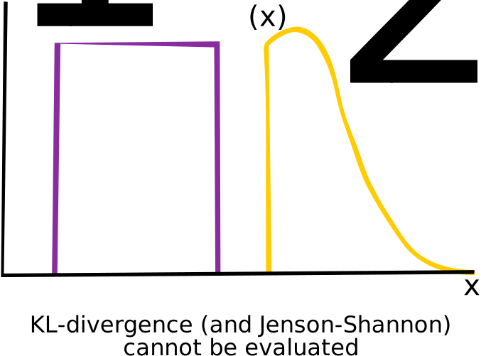
Wasserstein distance - approximate optimal transport using neural networks
Can we calculate the optimal way to transport a pile of dirt to another one (somewhere else) with a different shape?
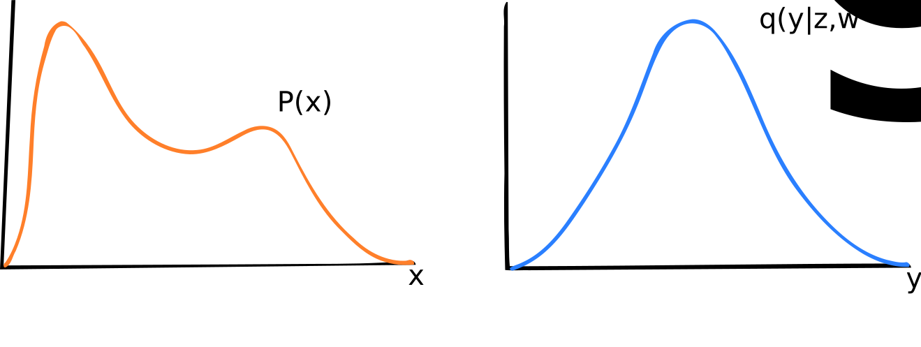
Why a pile of dirt?
- This was the original question asked my Monge nearly 250 years ago
We can now think of this pile of dirt as a probability distribution, i.e. probability mass spread over some events
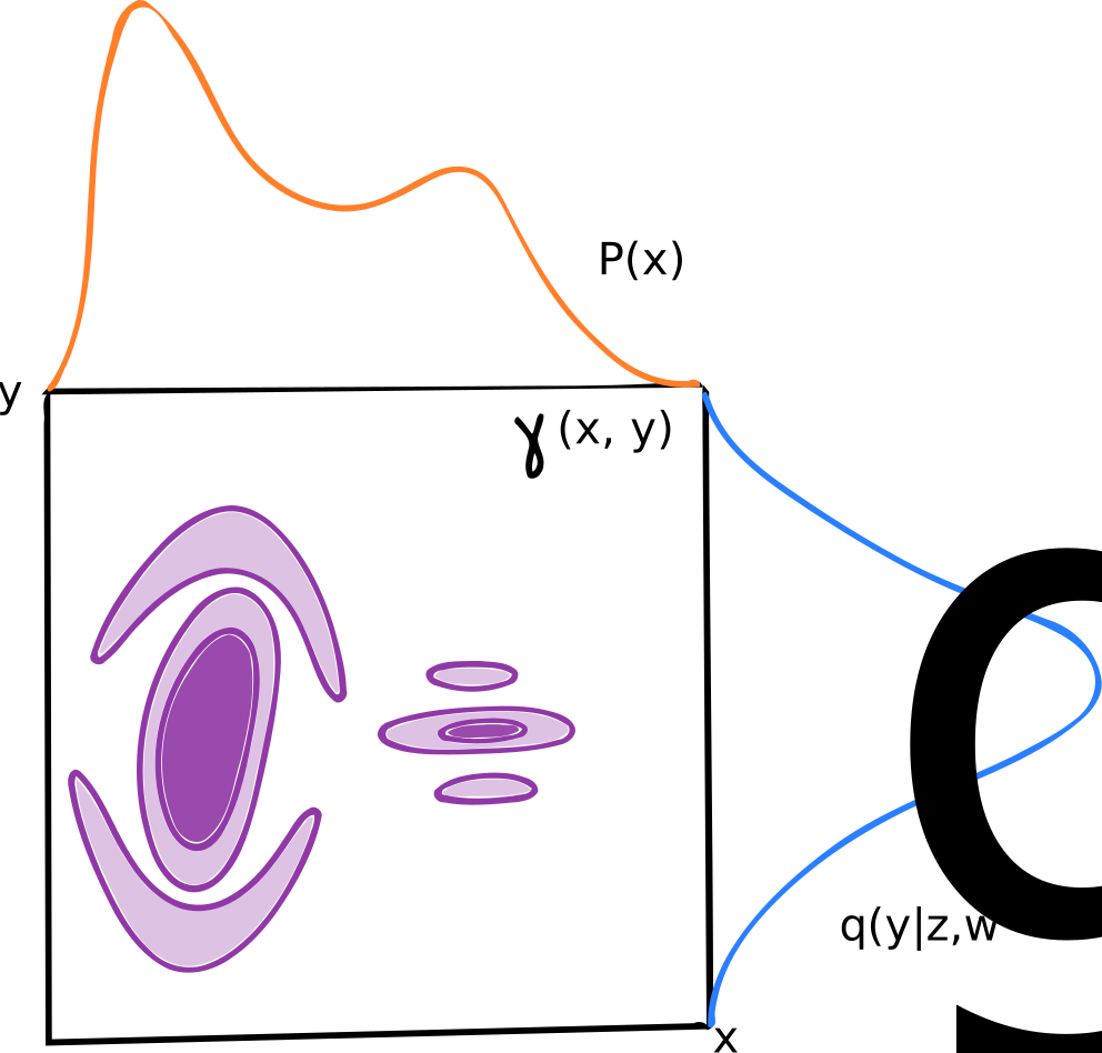
Distance function
$$E=\int_{E_x}\int_{E_y}dxdy\,\gamma(x,y)\|x-y\|$$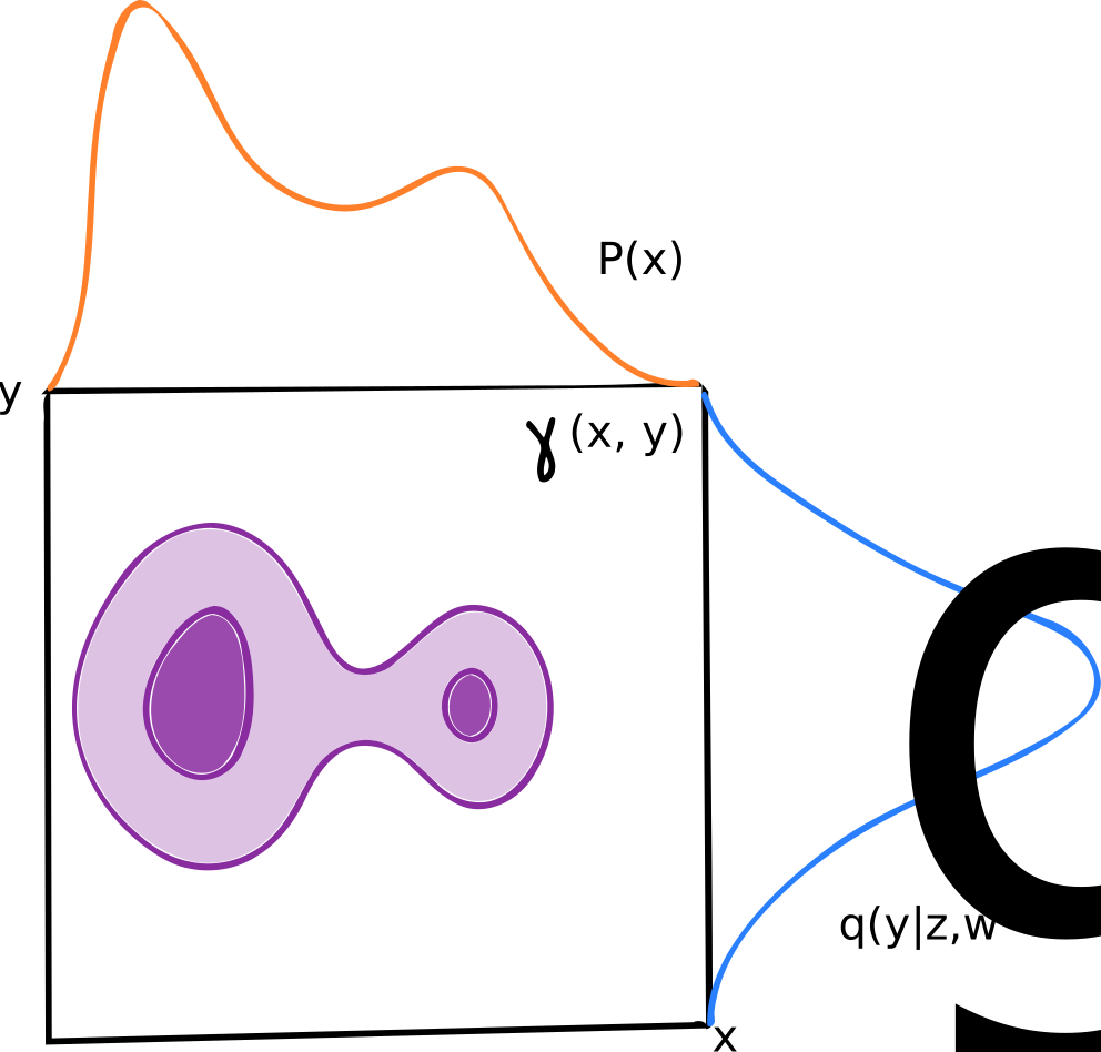
Smallest value of \\(E\\) for any \\(\gamma(x,y)\\) is the Earth mover distance
(or 1-Wasserstein distance - if using Euclidean distance)
Kantorovich-Rubinstein duality
$$W(P(x),{q(y|z,w^g,a^g)}) = \inf_{\gamma\in\Pi(P(x),{q(y|z,w^g,a^g)})}\int_{E_x}\int_{E_y}dxdy\,\gamma(x,y)\|x-y\|$$- Free up possible forms of $\gamma(x,y)$ and enforce constraint as $$\begin{align*} W(P(x),q(y|z,w^g,a^g)) &= \inf_\gamma\int_{E_x}\int_{E_y}dxdy\,\gamma(x,y)\left[\|x-y\|\right.\\ &\phantom{one}\left.+\sup_{f_{w^c,a^c},s}\left\{\int_{E_m}dm\,P(x)f_{w^c,a^c}(m)+\int_{E_m}dm\,q(y|z,w^g,a^g)s(m)-(f_{w^c,a^c}(x)-s(y))\right\}\right]. \end{align*}$$
If $\gamma(x,y)\in\Pi(P(x),q(y|z,w^g,a^g))$ then
$$\int_{E_x}\int_{E_y}dxdy\,\gamma(x, y)\left[\int_{E_m}dm\,P(x)f_{w^c,a^c}(m)+\int_{E_m}dm\,q(y|z,w^g,a^g)s(m)\right]=\int_{E_x}\int_{E_y}dxdy\,\gamma(x,y)(f_{w^c,a^c}(x)-s(y))$$For any sensible choice of $f_{w^c,a^c}$ and $s$, taking the supremum over $f_{w^c,a^c}$ and $s$ is infinity otherwise.
Thanks to the minimax principle we can take the supremum outside of the integral (and actually swapped with the infinimum) giving us
$$\begin{align*} W(P(x),q(y|z,w^g,a^g)) &= \sup_{f_{w^c,a^c},s}\inf_\gamma\int_{E_x}\int_{E_y}dxdy\,\gamma(x,y)\left[\|x-y\|-f_{w^c,a^c}(x)+s(y)\right.\\ &\phantom{one}\left.+\int_{E_m}dm\,P(x)f_{w^c,a^c}(m)+\int_{E_m}dm\,q(y|z,w^g,a^g)s(m)\right] \end{align*}$$
Taking the infinimum if $f_{w^c,a^c}(x)+s(y)\le K\|x-y\|$ then gives us
where $K$ is a constant.
We have managed to get rid of the transport plan $\gamma(x, y)$ completely!
But what are $f_{w^c,a^c}$ and $s$?
Since for all $x$ and $y$, $f_{w^c,a^c}(x)+s(y)\le K\|x-y\|$, for any positive constant, $K$ then $s(y)\le\inf_x K\|x-y\|-f_{w^c,a^c}(x)$.
The largest supremum possible occurs when $s(y)=\inf_x K\|x-y\|-f_{w^c,a^c}(x)$.
Choosing $f_{w^c,a^c}$ to be a $K$-Lipschitz function, i.e. $f_{w^c,a^c}(x)-f_{w^c,a^c}(y)\le K\|x-y\|$ has the advantage that $s(y)=\inf_x K\|x-y\|-f_{w^c,a^c}(x)$ is $K$-Lipschitz too.
We can therefore write $|s(y)-s(x)|\le K||y-x||$ which means
$$-K||x-y||\le s(y)-s(x)\le K||x-y||$$or equivalently
$$-s(x)\le K||y-x||-s(y).$$Since this is true for all $x$ then this means $$\begin{align*} -s(x)&\le\inf_y K||y-x||-s(y)\\ &\le f_{w^c,a^c}(x)\\ &\ge -s(x) \end{align*}$$ so we find that $f_{w^c,a^c}(x)=-s(x)$.
But machine learning...
By the way I have written this function, $f_{w^c,a^c}$, it's clear that we're going to approximate the $K$-Lipschitz functions using neural networks.
To make sure our network is a $K$-Lipschitz function, we need to make sure its norm does not get bigger than $K$ - in fact we don't really care what value $K$ since it just causes a scaling of the Wasserstein distance.
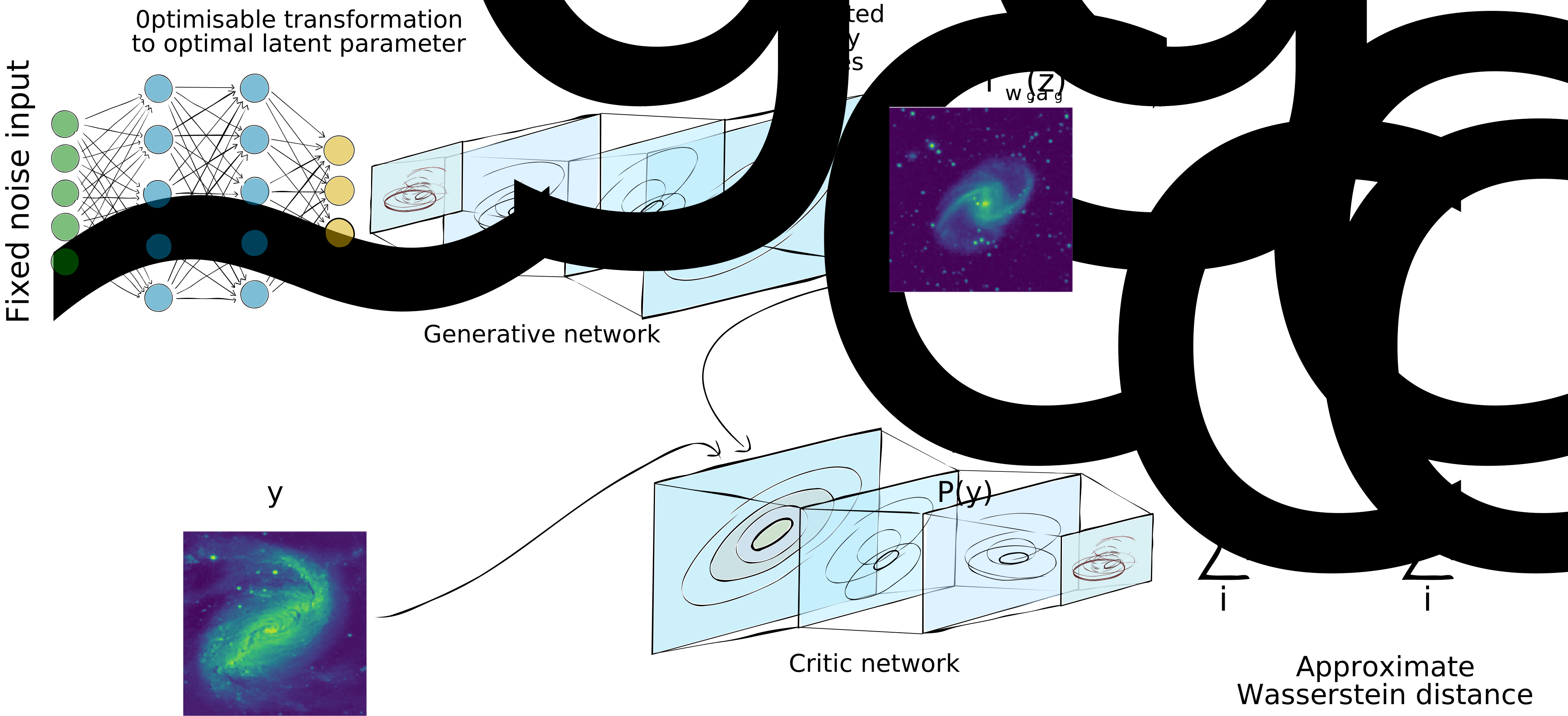
So we can approximise the Wasserstein distance simply by maximising the difference between the output of the neural network with a sample drawn from the first distribution, $y\sim P(y)$, and with a sample drawn from the second distribution $Y\sim q(Y|z,w^g,a^g)$
$$W(P(y),q(Y|z,w^g,a^g)) \propto \max_{w^c\in E_{w^c}}\sum_{i=1}^{n_\textrm{train}}f_{w^c,a^c}(y_i)-\sum_{i=1}^{n_\textrm{train}}f_{w^c,a^c}(Y_i)+\lambda\sum_{i=1}^{n_\textrm{train}}(||\nabla_{\hat{y}}f_{w^c,a^c}(\hat{y}_i)||-1)^2$$where $\hat{y}=\epsilon y + (1-\epsilon) Y$ where $\epsilon\sim\textrm{Uniform}[0, 1]$ and $\lambda$ is a coupling strength to the norm regularisation.
By optimising $w^c$ we can get a good approximation to the Wasserstein distance which we can then use to optimise ANOTHER neural network!
Wasserstein GAN
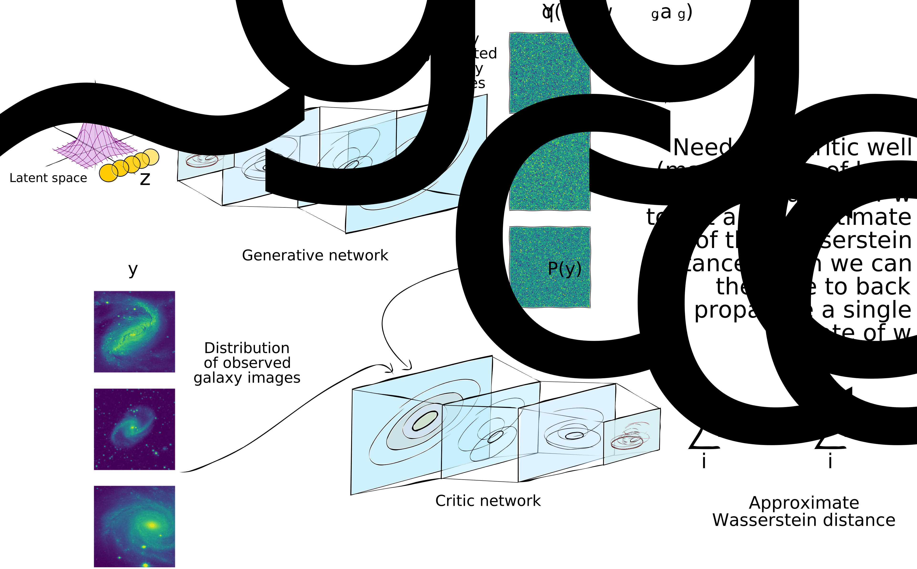
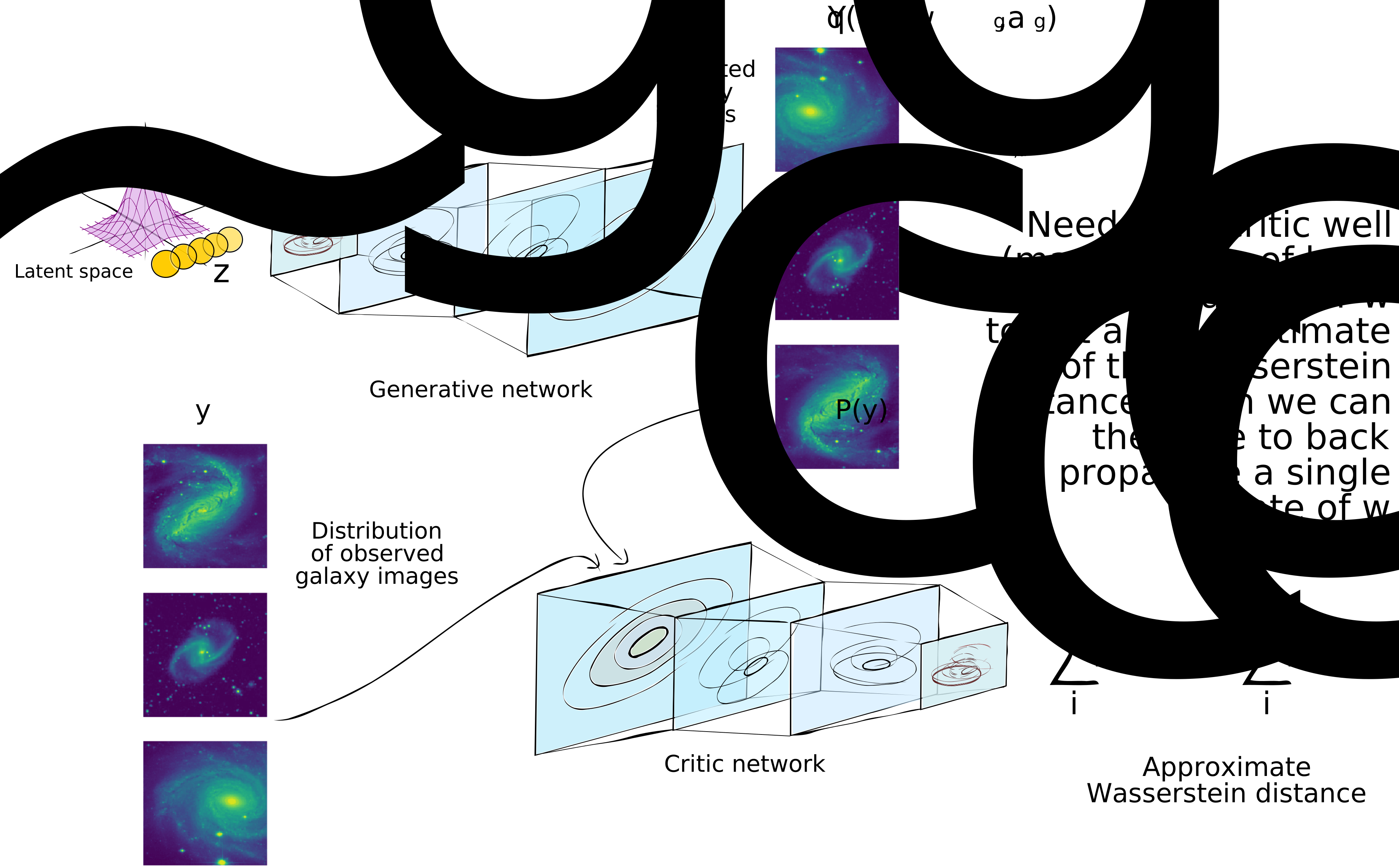
Side note - generative networks and adversarial training
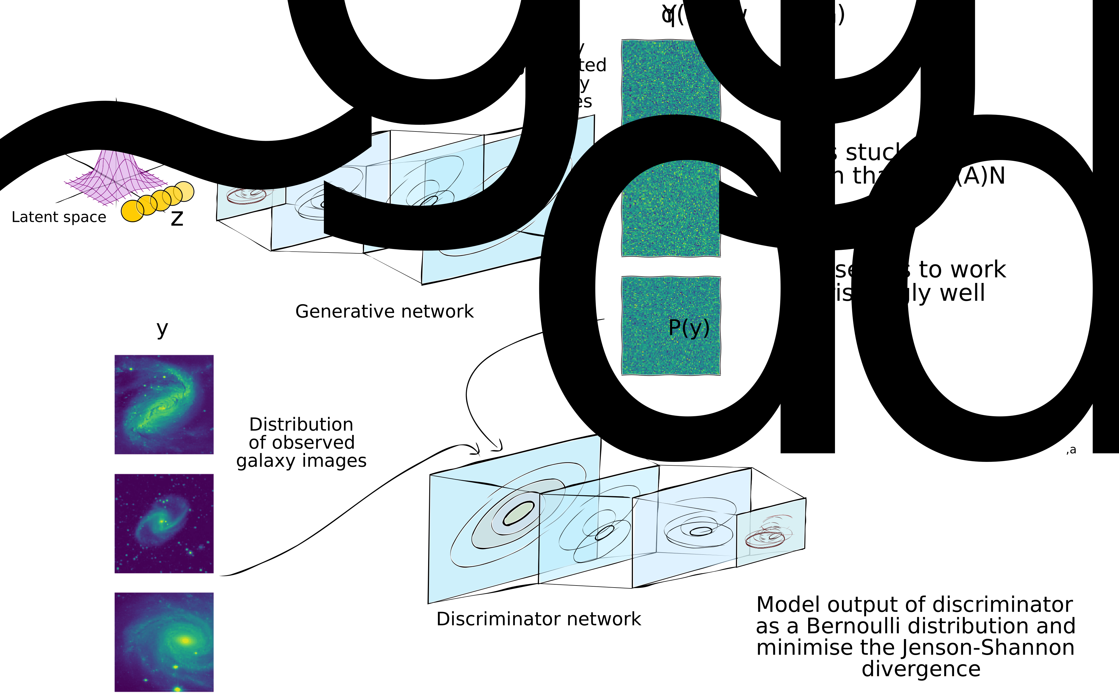
Try to reach a Nash equilibrium (where adversarial word comes from)
Another example
rng, key = jax.random.split(rng)
_, initial_params = dense_predictor.init_by_shape(
key, [((100,), np.float64)])
W_model = flax.nn.Model(dense_predictor, initial_params)
W_opt = flax.optim.Adam(1e-5).create(W_model)
@jax.jit
def wasserstein_distance(y, y_pred, model):
return np.mean(model(y)) - np.mean(model(y_pred))
def W_vae_loss(model, W_model, key, samples=10):
def get_loss(y_pred, loc, log_scale):
return np.mean(np.mean(W_model(y_pred)) - KL(loc, log_scale))
y_pred, loc, log_scale = model(y_train, samples=samples, key=key)
return jax.jit(get_loss)(y_pred, loc, log_scale)
def W_loss(y_pred, model, λ, key):
def norm(y_):
return np.linalg.norm(model(y_))
ϵ = jax.random.uniform(key, shape=y_pred.shape[:-1] + (1,))
y_hat = ϵ * y_train[:, np.newaxis] + (1 - ϵ) * y_pred
return wasserstein_distance(y_train, y_pred, model) + np.mean(λ * (jax.grad(norm)(y_hat)-1)**2)
def W_vae_optimise(vae_opt, W_model, key, samples=10):
vae_grad = jax.grad(lambda model : W_vae_loss(model, W_model, key=key, samples=samples))(vae_opt.target)
vae_opt = vae_opt.apply_gradient(vae_grad)
return vae_opt
def W_optimise(W_opt, vae_model, rng, λ=10, samples=10):
rng, key = jax.random.split(rng)
y_pred, _, _ = vae_model(y_train, samples=samples, key=key)
rng, key = jax.random.split(rng)
W_grad = jax.grad(lambda model : W_loss(y_pred, model, λ, key))(W_opt.target)
W_opt = W_opt.apply_gradient(W_grad)
return W_opt, rng
if os.path.isfile("data/W_opt.npy"):
epochs = 5
vae_opt = flax.serialization.from_state_dict(vae_opt, np.load("data/W_vae_opt.npy", allow_pickle=True)[()])
W_opt = flax.serialization.from_state_dict(W_opt, np.load("data/W_opt.npy", allow_pickle=True)[()])
W_KL_ = [i for i in np.load("data/W_KL.npy")]
val_W_KL_ = [i for i in np.load("data/val_W_KL.npy")]
W_ = [i for i in np.load("data/W.npy")]
val_W_ = [i for i in np.load("data/val_W.npy")]
else:
epochs = 150
W_KL_ = []
val_W_KL_ = []
W_ = []
val_W_ = []
bar = tqdm.tnrange(epochs, desc="iterations"); critic_epochs = 5
for i in bar:
for j in range(critic_epochs):
W_opt, rng = W_optimise(W_opt, vae_opt.target, rng, λ=10, samples=10)
rng, key = jax.random.split(rng)
y_pred, _, _ = vae_opt.target(
y_train, samples=1, key=key)
W_.append(wasserstein_distance(y_train, y_pred, W_opt.target))
rng, key = jax.random.split(rng)
y_pred, _, _ = vae_opt.target(
y_validate, samples=1, key=key)
val_W_.append(wasserstein_distance(y_validate, y_pred, W_opt.target))
rng, key = jax.random.split(rng)
vae_opt = W_vae_optimise(vae_opt, W_opt.target, key, samples=10)
rng, key = jax.random.split(rng)
_, loc, log_scale = vae_opt.target(
y_train, samples=1, key=key)
W_KL_.append(np.mean(KL(loc, log_scale)))
rng, key = jax.random.split(rng)
_, loc, log_scale = vae_opt.target(
y_validate, samples=1, key=key)
val_W_KL_.append(np.mean(KL(loc, log_scale)))
bar.set_postfix(KL=W_KL_[-1], val_KL=val_W_KL_[-1],
W=W_[-1], val_W=val_W_[-1])
#np.save("data/W_KL.npy", W_KL_);np.save("data/val_W_KL.npy", val_W_KL_);np.save("data/W.npy", W_);np.save("data/val_W.npy", val_W_);np.save("data/W_opt.npy", flax.serialization.to_state_dict(W_opt));np.save("data/W_vae_opt.npy", flax.serialization.to_state_dict(vae_opt))
fig, ax1 = subplots(figsize=(20, 16)); ax2 = ax1.twinx(); labels = ["Training KL", "Validation KL", "Training W", "Validation Training W"];ax1.set_xlabel("Epochs", fontsize=20);ax1.set_ylabel("KL divergence", fontsize=20);ax2.set_ylabel("W", fontsize=20);ax1.tick_params(axis="both", labelsize=20); ax2.tick_params(axis="both", labelsize=20); epo3 = np.arange(1, len(W_KL_)+1)
a = ax1.plot( W_KL_, linewidth=3)
b = ax1.plot( val_W_KL_, linewidth=3)
c = ax2.plot( W_, linestyle="dashed", linewidth=3)
d = ax2.plot( val_W_, linestyle="dashed", linewidth=3)
legend(a+b+c+d, labels, fontsize=20);

rng, key = jax.random.split(rng)
W_trained_y_mean, W_trained_loc, W_trained_log_scale = vae_opt.target(y_test)
W_trained_y_gen, _, _ = vae_opt.target(y_test, samples=10, key=key)
figure("Trained generated samples", figsize=(24, 16)); xlabel("$f_{w_\mu^e,a_\mu^e}(x)$", fontsize=20); ylabel("$f_{w_\Sigma^e,a_\Sigma^e}(x)$", fontsize=20);tick_params(axis="both", labelsize=20)#;yscale("log");ylim([1e-19, 100])
scatter(W_trained_loc[:, 0], W_trained_log_scale[:, 0], c=m_test[:, 0])
cbar = colorbar(); cbar.set_label("m", fontsize=20); cbar.ax.tick_params(labelsize=20)

figure("Trained generated samples", figsize=(20, 16)); xlabel("x", fontsize=20); xlim([0.11, 10]); ylabel("y train", fontsize=20);tick_params(axis="both", labelsize=20); ylim([-10, 40])
plot(x, W_trained_y_gen[3].T, linestyle="dotted", linewidth=3)
plot(x, W_trained_y_mean[3], color="black", label="Mean generated sample", linewidth=3)
plot(x, y_test[3], label="Target sample", linewidth=3)
legend(fontsize=20, frameon=False);

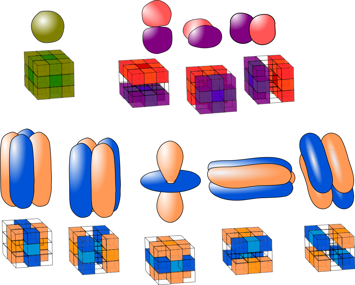
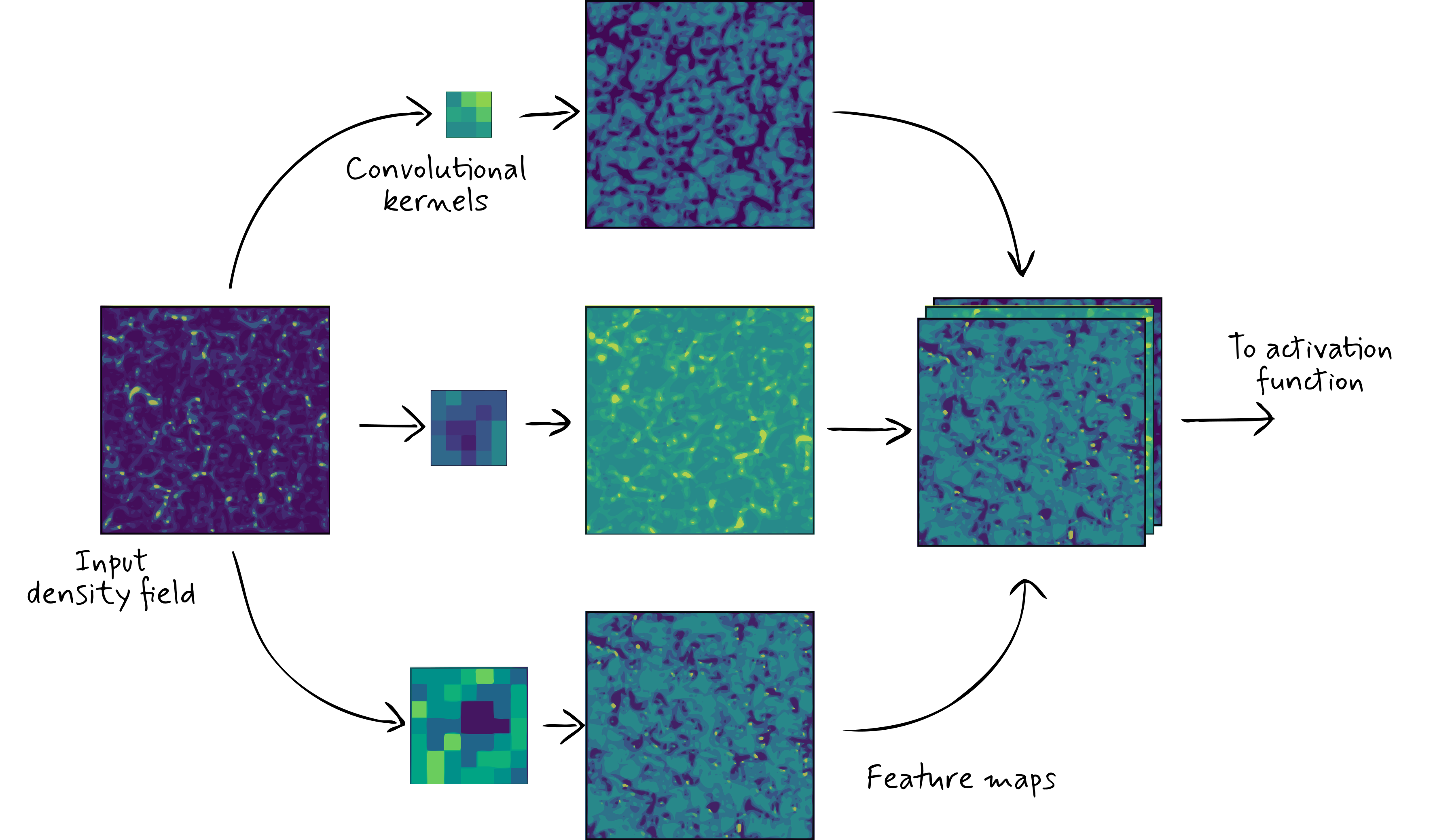
What features exist in cosmological and astrophysical data
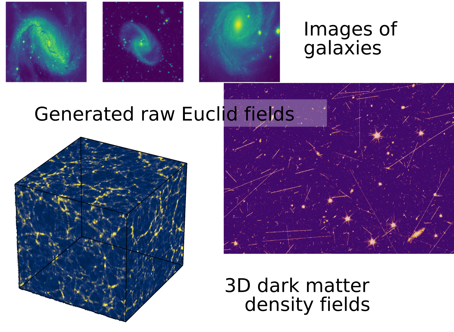
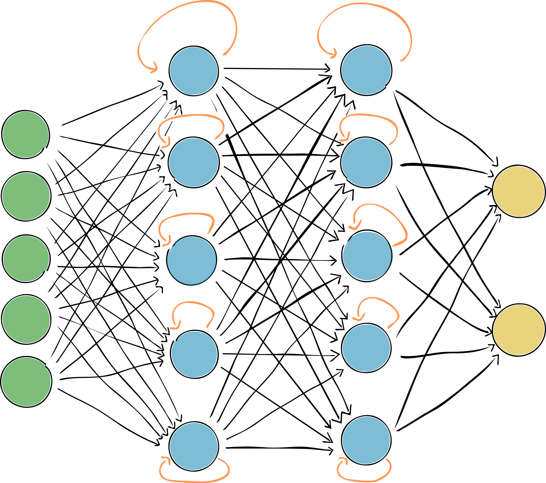
Ideal network architectures (actually doing different physics)
Building the function that best suits the data will cut down massively on training data, overfitting, time to convergence, and a whole lot of things (becomes less deep, but depth might not necessarily be useful for our purpose).
It does cost you a bit of extra brain power...
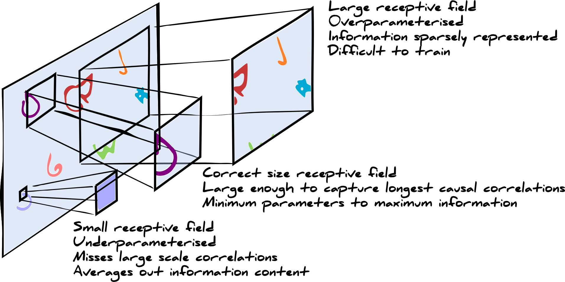
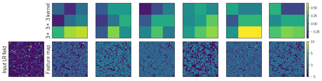
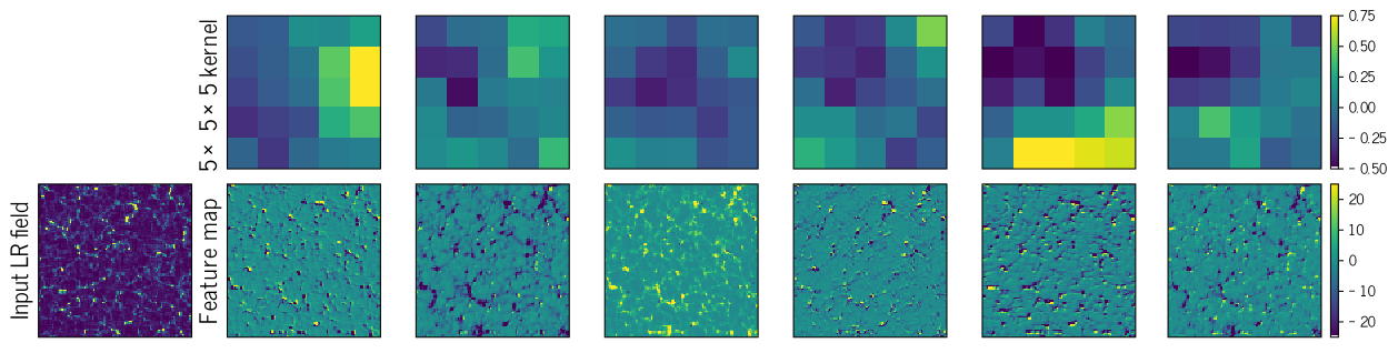
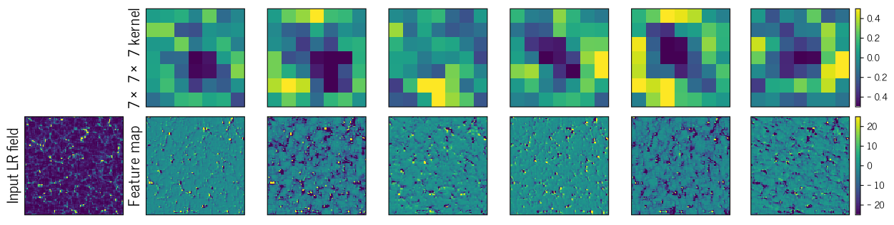
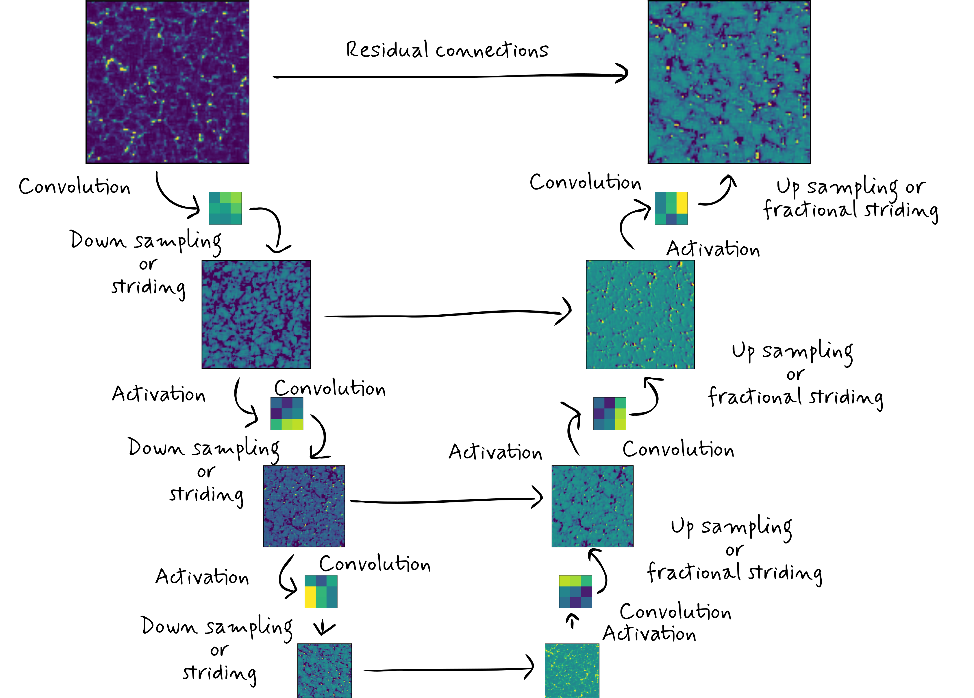
U-net
Inception
Example 1 : Calibration of the VIS CCD
(Bretonniere, Charnock, McCracken)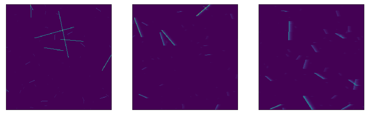
We could try and just predict the numbers, but why would we trust our model, when we don't know the model!?
Instead we can learn the distribution of data using a conditional WGAN (VAE with a Wasserstein metric)
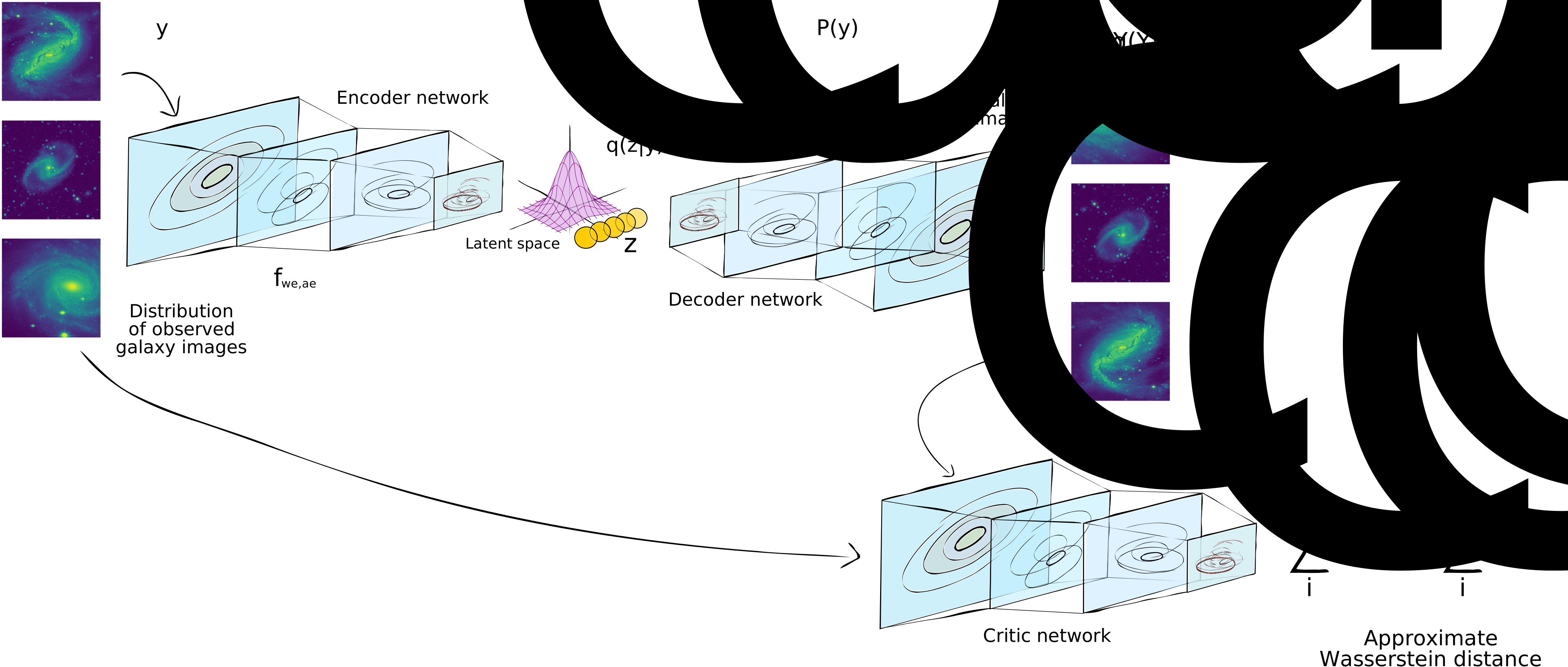
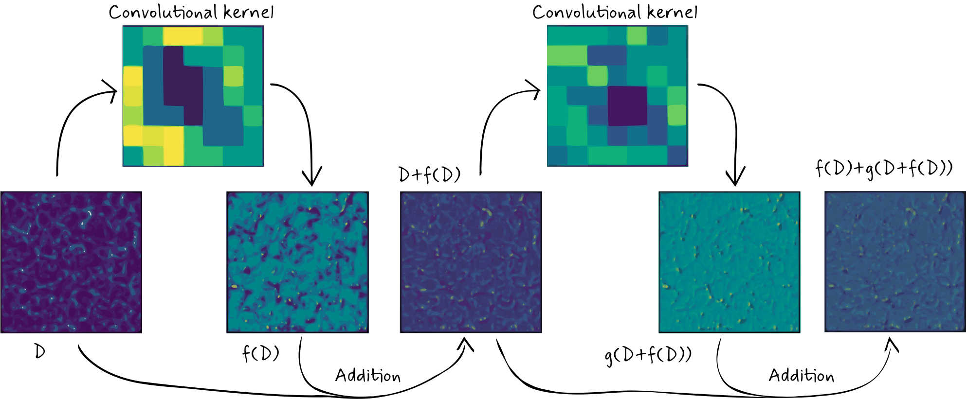
Inception with residual connections
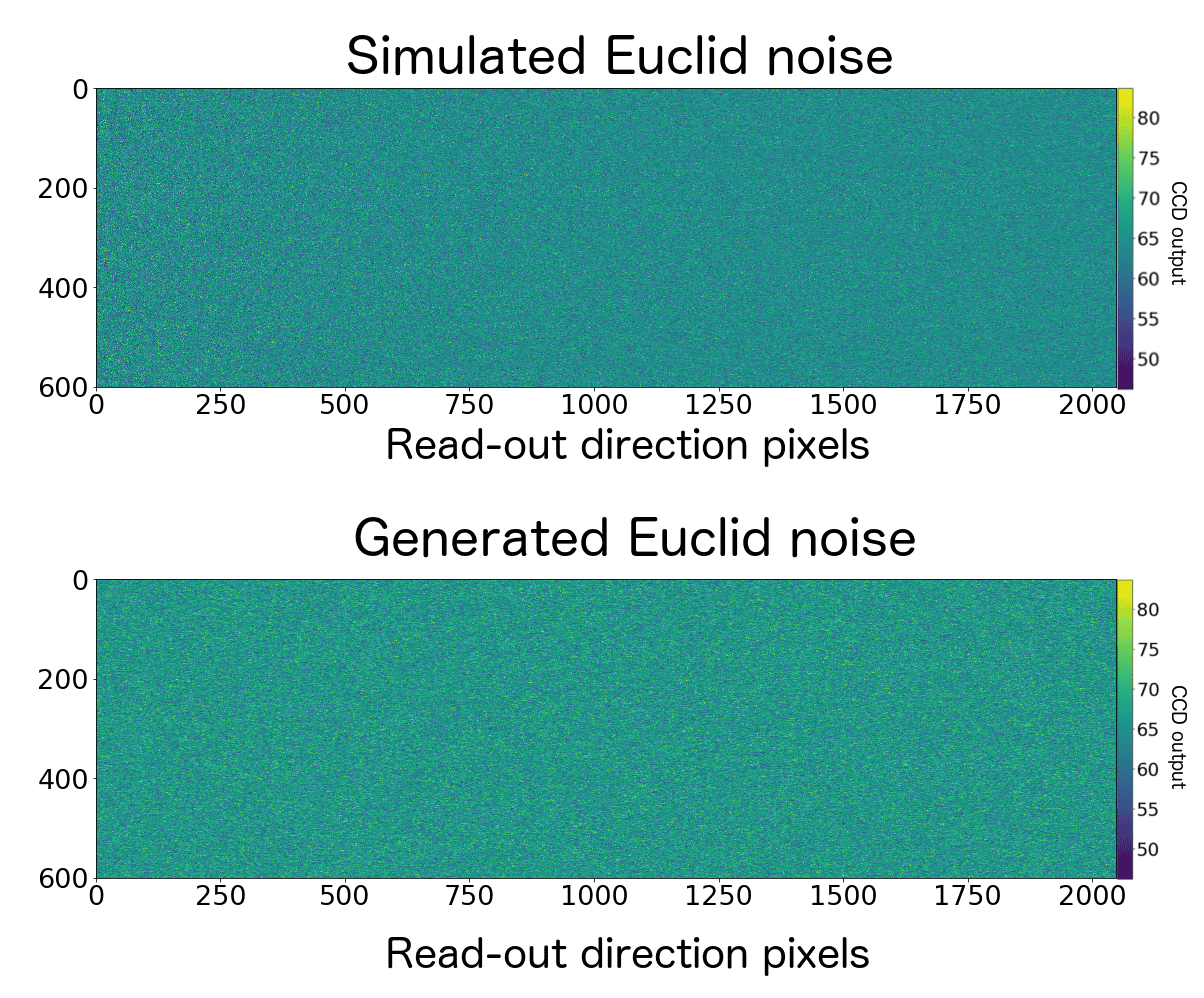
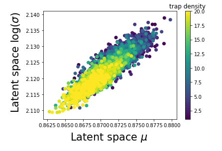
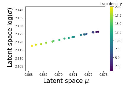
We can effectively correlate the parameter values with the variational distribution
Example 2 : Finding out-of-distribution objects
(Margalef-Bentabol, Huertas-Company, Charnock, Margalef-Bentabol, Bernardi, Dubois, Storey-Fisher, Zanisi 2020)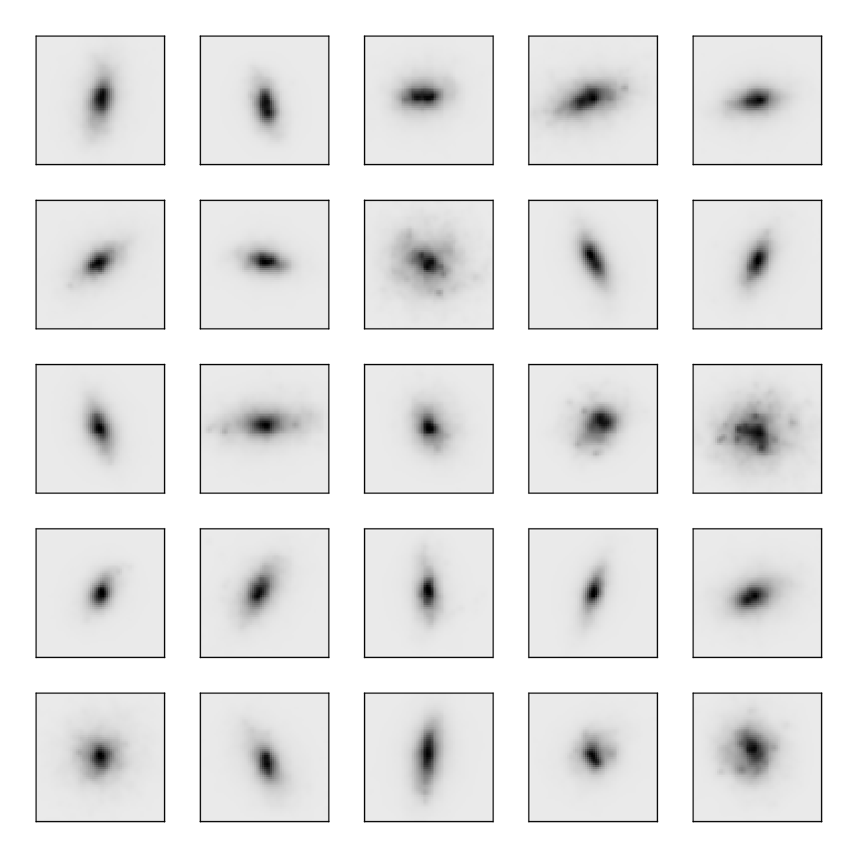
Can we learn the distribution of expected galaxy types?
Use the Horizon-AGN simulation
Compare to CANDELs to identify objects that are not seen in Horizon-AGN
Look at the properties of the out-of-distribution objects to see what is missing in simulations
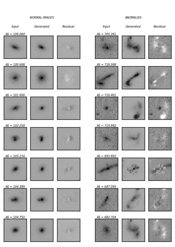
What did we use to generate similar images?
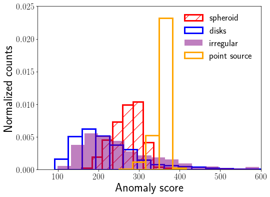
Calculate anomaly scores and comparison of results
- Anomaly scores are small for in-distribution objects because we can generate similar images
- Anomaly scores are larger for out-of-distribution objects because we cannot generate similar images
Comparing the distribution of anomaly scores to the generated set gives us anomaly detection of images an properties
Example 3 : Generating accelerated simulations
(Zhang, Wang, Zhang et al., 2019)
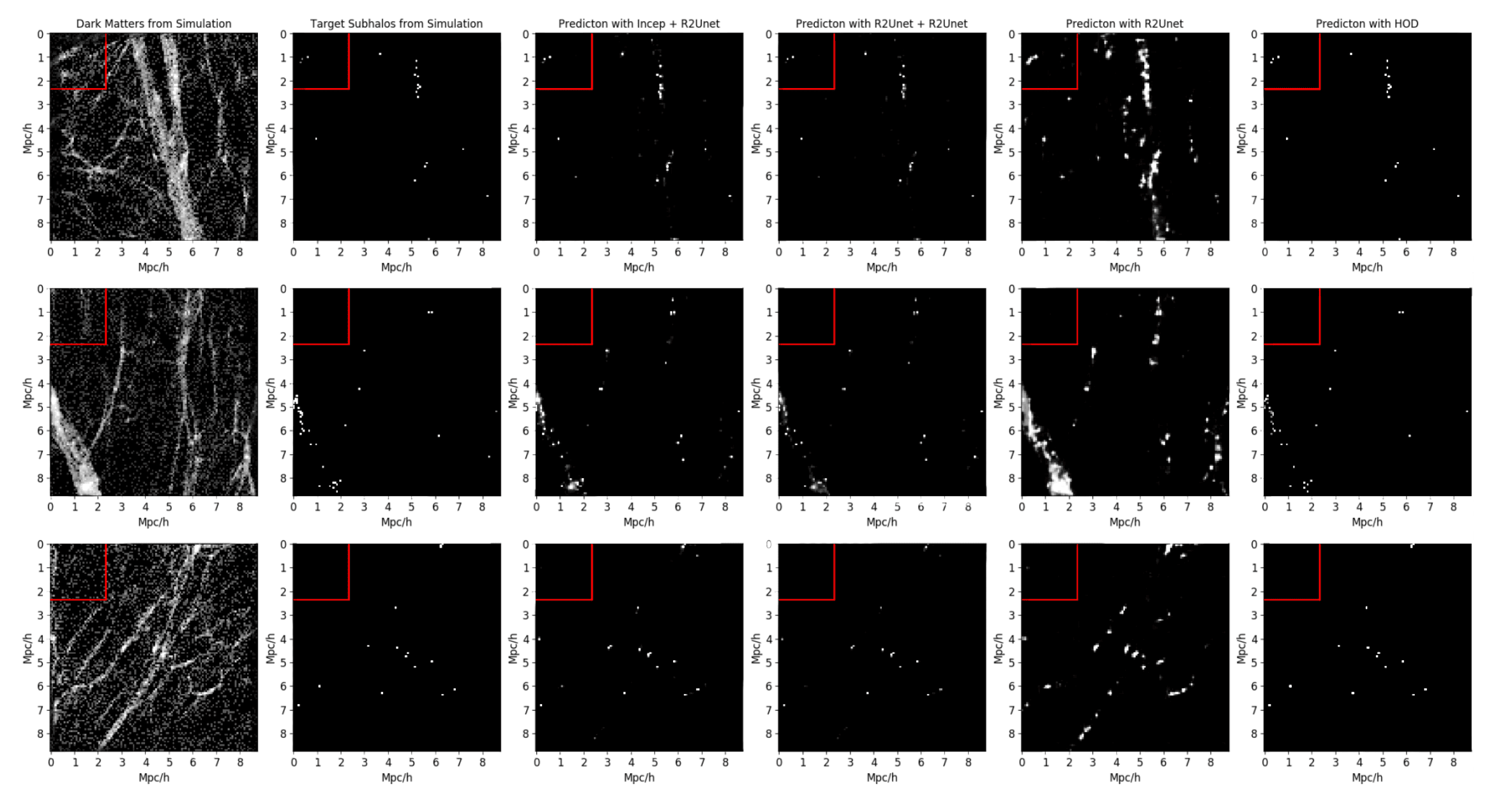
Using U-map to pull out features at all scales
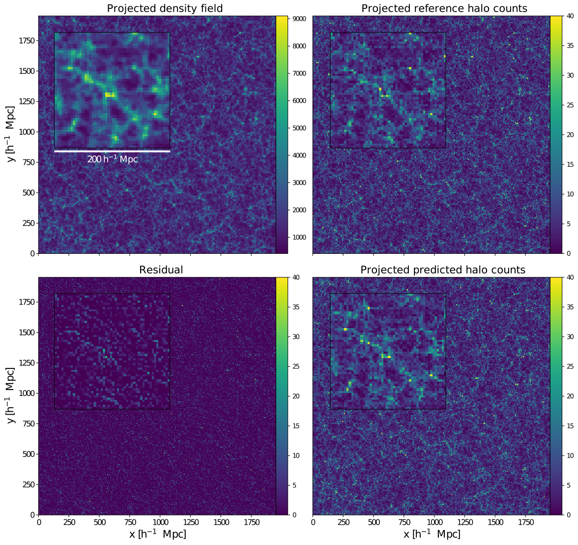
Physically motivated functions
(Doogesh Kodi Ramanah, Tom Charnock and Guilhem Lavaux 2019)
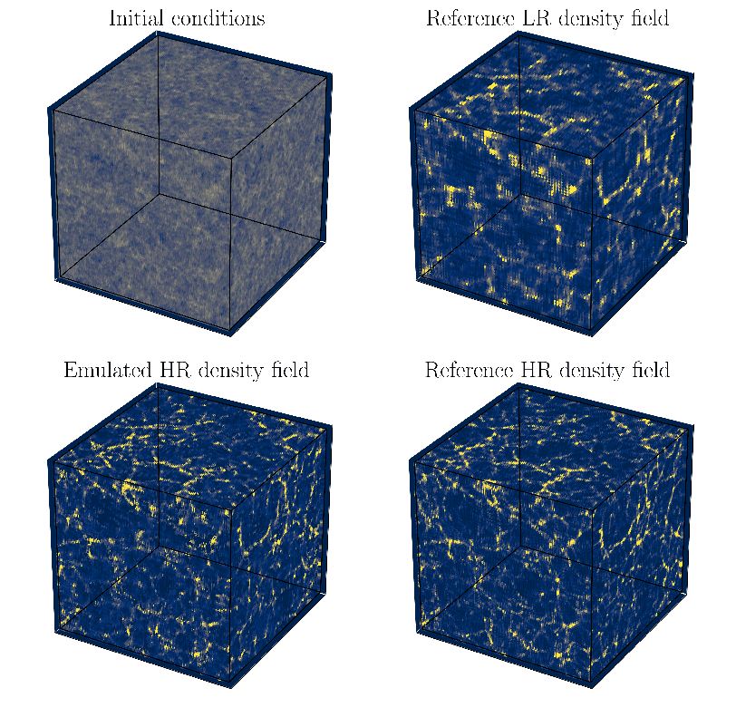
Superresolution emulation
(Doogesh Kodi Ramanah, Tom Charnock, Francisco Villaescusa-Navarro and Benjamin D. Wandelt 2020)
Caveats
These simulations are not as safe as performing true N-body simulations
- we do not actually know that the generated data is really "in"-distribution.
- their expectation values should be very close to the expectation value of the true N-body
We cannot use them to do cosmological parameter estimation by forward simulation
We can use them to make very very good Fisher estimates, very very quickly
Statistical methods
Bayesian neural networks
Describe weights as $$p(w|x,y,a) = \frac{L(y|x,w,a)p(w|a)}{p(D|a)}$$
And calculate error using $$p(y|x)=\int_{E_a}\int_{E_w}dadw\,L(y|x,w,a)p(w|x_\textrm{train},y_\textrm{train}, a)p(a)$$
Beyond loss function stochastic models
- We have so far chosen a loss function which is really the description of the likelihood in our statistical model
We can attempt to fit the posterior with much more complex distributions by inferring the distribution of network weights $p(w|x_\textrm{train},y_\textrm{train},a)\approx q(w|x_\textrm{train},y_\textrm{train},a)$ and calculating
$$p(y|x)=\int_{E_a}\int_{E_w}dadw\,L(y|x,w,a)p(w|x_\textrm{train},y_\textrm{train}, a)p(a)$$This allows for much more abstract distributions, $q(y|x,w,a)\approx P(y|x)$, to be fitted using variational inference.
Note
Current methods described as Bayesian neural networks are not very "Bayesian"
- Distribution is chosen is chosen for the weights and $P(y|x)$ is fitted.
- Quick to train (in general), but there is no certainty about how good the fit is.
In essence there is no difference between a classically trained neural network and what people are calling a Bayesian neural network.
You can have actual Bayesian neural networks where there is no variational assumption on these weights, but these have a lot of other caveats (Charnock, Lavaux, Wandelt, Sarma Boruah, Jasche & Hudson 2020)
Bayes by backprop
Reparameterisation trick
$$\begin{align*} w_i&\sim q(w_i|x_\textrm{train},y_\textrm{train},a)\\ &\equiv\mathbb{N}(\mu_i,\sigma_i)\\ &=\mu_i+\sigma_i\epsilon_i \end{align*}$$where $\epsilon_i\sim\mathbb{N}(0, 1)$ where $i\in[1, n_\textrm{weights}]$.
Calculate $\textrm{ELBO}(q(y|x,w,a))$ and then maximise it using backpropagation for the parameters of the (Gaussian) weight distribution
$$\begin{align*} \mu_i &\leftarrow \mu_i - \eta\left(\partial_{w_i}\textrm{ELBO}(q(y|x,w,a)) + {\partial_{\mu_i}}\textrm{ELBO}(q(y|x,w,a))\right)\\ \sigma_i&\rightarrow \sigma_i-\eta\left(\frac{\epsilon_i}{\sigma}\partial_{w_i}\textrm{ELBO}(q(y|x,w,a)) + {\partial_{\sigma_i}}\textrm{ELBO}(q(y|x,w,a))\right) \end{align*}$$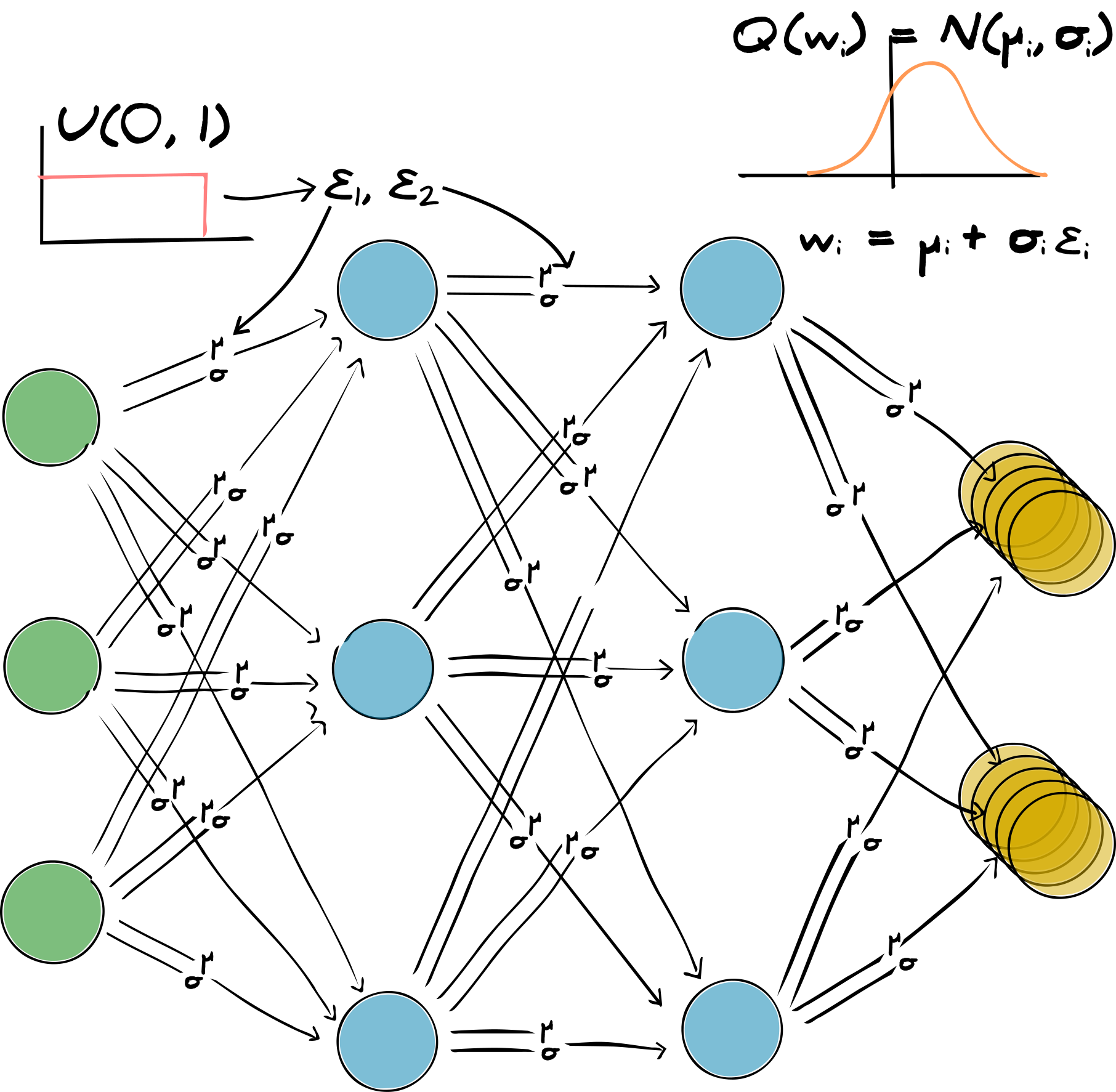
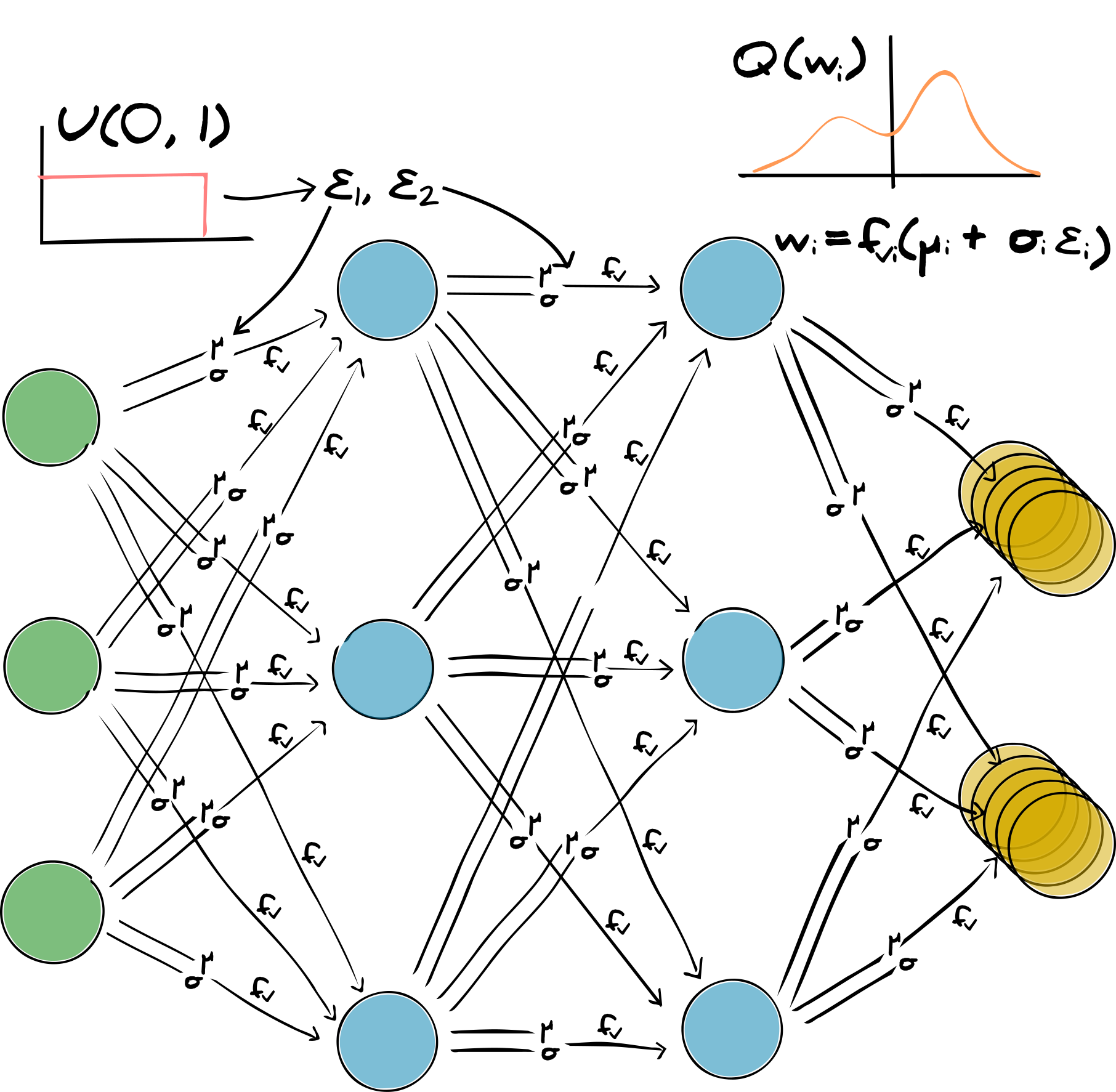
Impracticalities of BbB
$\epsilon$ needs to be drawn for every weight in the network and every element of data in the training set.
This is normally too expensive to actually store using modern hardware or makes computation extremely slow
So we assume just one epsilon for each weight
This is a poor representation of the distribution of parameters and so there is an artificially high variance in the stochastic gradient.
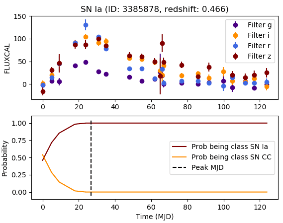
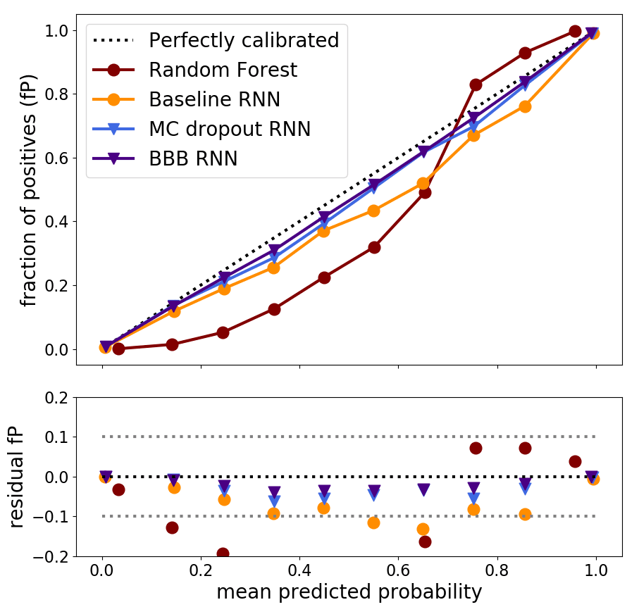
Example 4 : Classification of supernovae type from photometric lightcurves (SuperNNova)
(Möller & Boissiere, 2019)
Recurrent neural network (time series) + Bayes by backprop
Local reparameterisation trick
Model neuron output as $$o_{jn}^l=\sum_{i=1}^{\textrm{dim }l-1}\mu_{ji}^la_{in}^{l-1}+\epsilon_{jn}^l\sqrt{(\sigma_{ji}^l)^2(a_{in}^{l-1})^2}$$
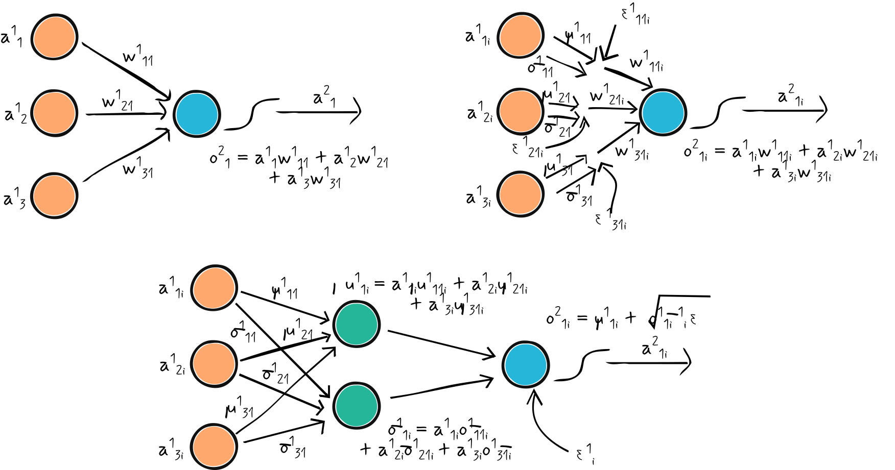
$n_\epsilon$ in BbB $n_\textrm{weights}\times n_\textrm{train}$ $n_\epsilon$ in LRT $n_\textrm{layer outputs}\times n_\textrm{train}$
Whether this is as good of an approximation or not is debatable, its definitely less relatable to the posterior distribution of weights $P(w|x,y,a)$
Variational dropout
Local reparameterisation only works when there is no weight sharing, i.e. it doesn't work for convolutional networks, etc.
We can, however, approximate distributions using multiplicative noise - variational dropout
$$a_{in}^l=\epsilon_{in}^l f(o_{in}^l)$$where $\epsilon_{in}^l\sim\textrm{Dist}(m_{(in)}^{(l)})$ for any distribution.
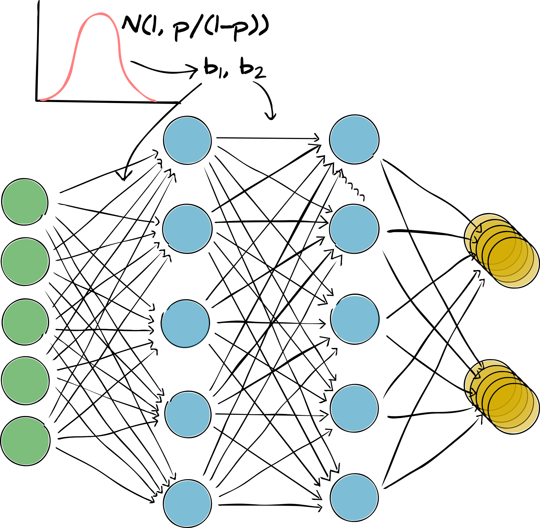
Bernoulli dropout ($\epsilon_{in}^l\sim\textrm{Bernoulli}(b_{(in)}^{(l)})$)
Gaussian dropout ($\epsilon_{in}^l\sim\mathbb{N}(1,b_{(in)}^{(l)})$)
MC Dropout
Train a neural network with dropout (a random dropping of layer outputs) with $\ell_2$ regularisation
equivalent to maximising the ELBO (real VI)
most popular method by far, because of speed and ease of implementation
Variational (and MC) dropout is a very poor representation of $P(w|x,y,a)$ because the distribution of weights isn't considered
- not very Bayesian.
Flipout
Alternative local reparameterisation trick
Symmetric perturbative distribution $w = \mu + \Delta w$ where $\Delta w\sim \textrm{SymDist}$
Draw 2 random vectors $j$ and $k$ of -1 and 1s for each weight and each element in training data
Pseudo-independent weight samples
$$w_{in}=\mu_i+\Delta w_i j_{in}k_{in}$$- Reduces the variance of stochastic gradient by a factor of $1/n_\textrm{elems}$
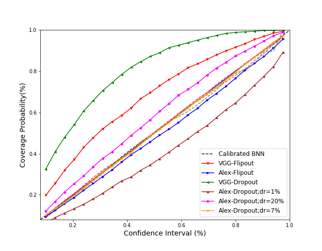
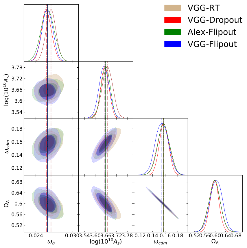
- Best results at the moment from variational inference.
Note that this might be a bad estimate of $P(w|x,y,a)$ because we have to assume that it is unimodal and symmetric - which is almost certainly not a good approximation of $P(w|x,y,a)$.
Neural networks using in a Bayesian setting
(Charnock, Lavaux, Wandelt, Sarma Boruah, Jasche and Hudson 2020)
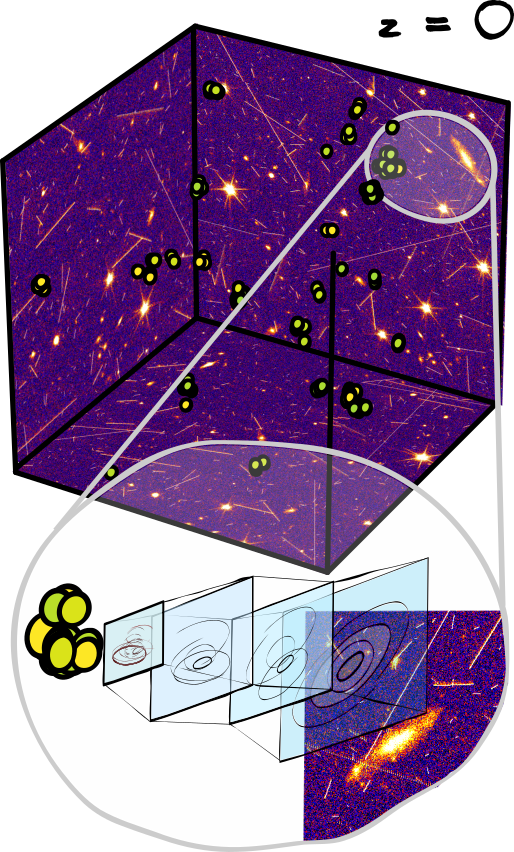
- Forward model all understood physics
- Make abstract function (NN) made from physically motivated architecture choice
- Remove all unidentifiable weights
- Use high dimensional Markov methods to sample physical properties AND neural network weights
Not deep learning anymore - we're just benefitting from the differentiable frameworks and doing old-school* physics 😉

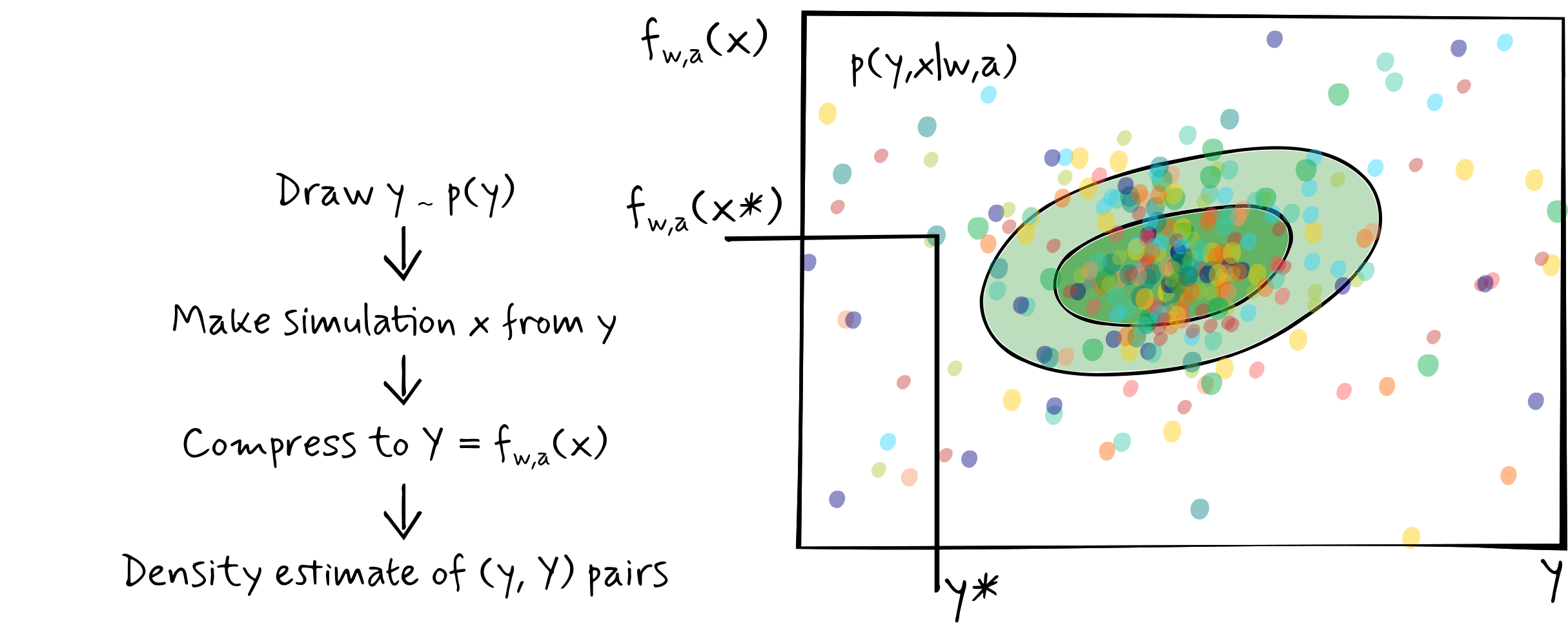
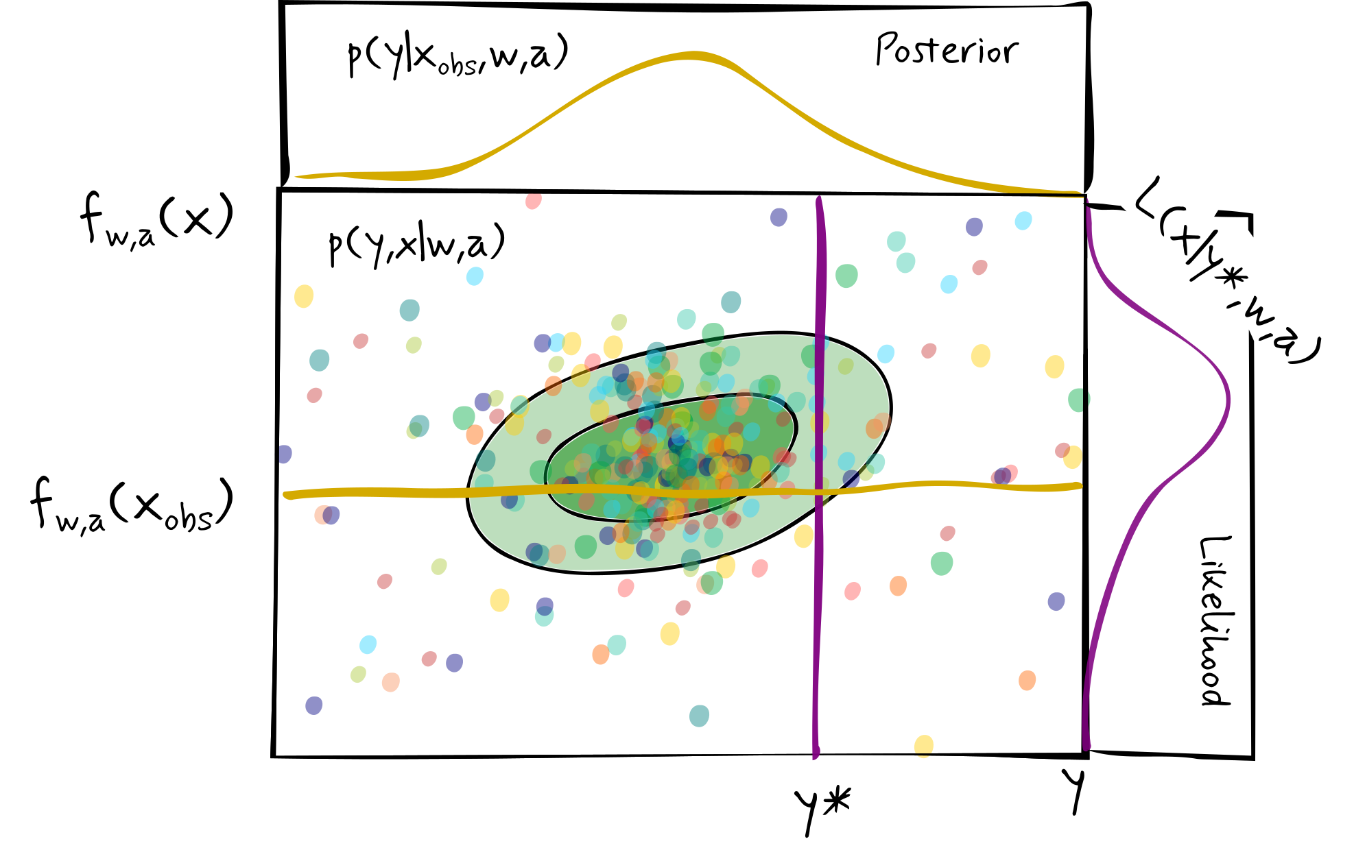
Approximate Bayesian computation (ABC)
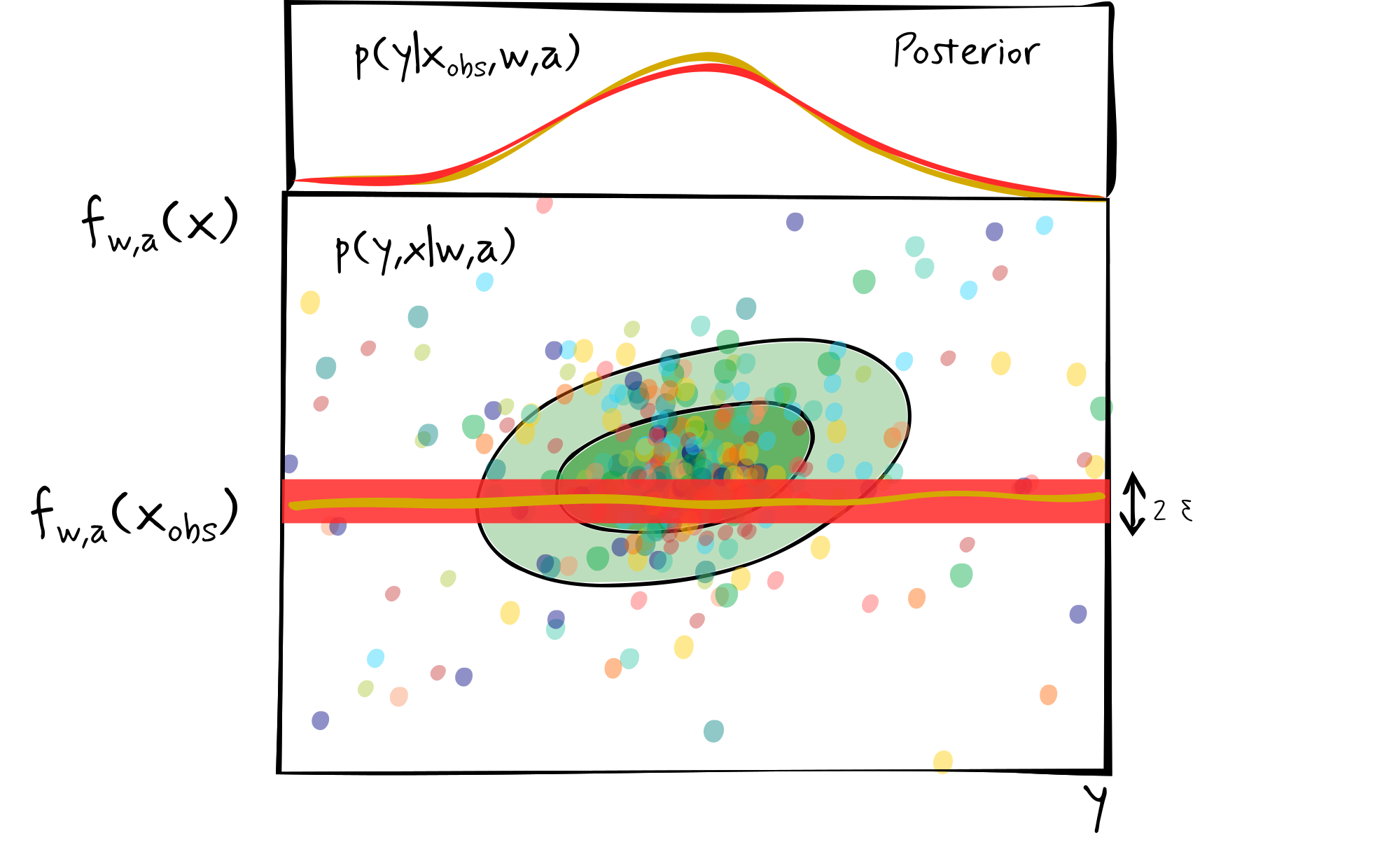
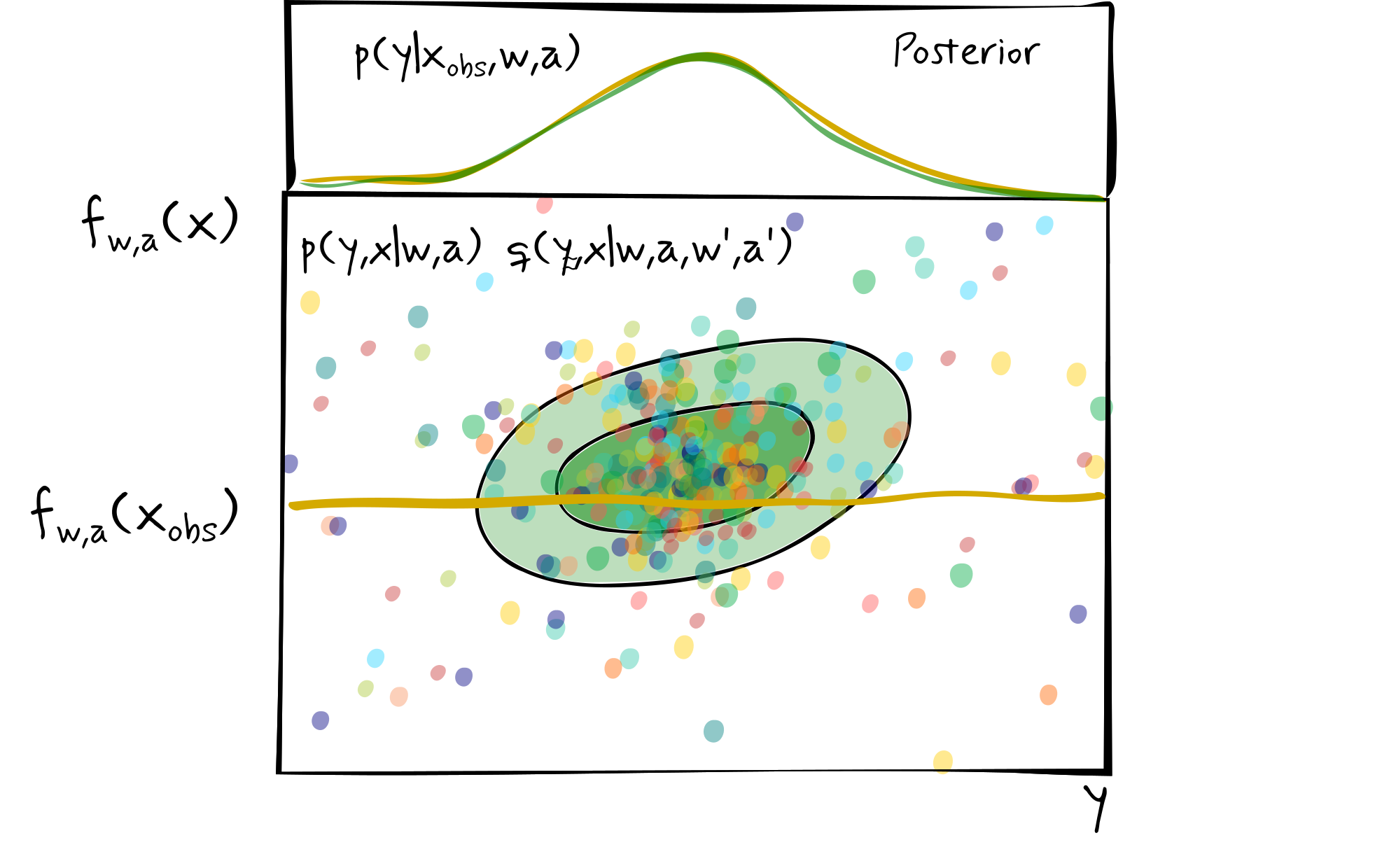
Density estimate likelihood-free inference (DELFI)
Another example - yay!
n_LFI = int(1e5)
rng, key = jax.random.split(rng)
m_LFI = jax.random.uniform(key, minval=-5, maxval=5, shape=(n_LFI, 1))
rng, key = jax.random.split(rng)
t_LFI = mse_opt.target(simulator(m_LFI, key))
DELFI_LFI = gaussian_kde(np.concatenate([m_LFI, t_LFI], axis=-1).T)
m_obs = m_test[3, 0]
t_obs = mse_opt.target(y_test[3])[0]
ϵ_LFI = 0.1
bins = 100
fig, ax = subplots(2, 2, figsize=(20, 20)); ax[0, 1].axis("off"); ax[1, 0].set_xlabel("m", fontsize=20), ax[1, 0].set_ylabel("t", fontsize=20);ax[1, 1].set_xlabel("L(t|m obs, w, a)", fontsize=20);ax[0, 0].set_ylabel("P(m|y obs, w, a)", fontsize=20);subplots_adjust(wspace=0, hspace=0);ax[0, 0].set_xticks([]);ax[1, 1].set_yticks([]);ax[0, 0].set_xlim([-5, 5]);ax[1, 0].set_xlim([-5, 5]);ax[1, 0].set_ylim([-5, 5]);ax[1, 1].set_ylim([-5, 5]);ax[0, 0].tick_params(axis="both", labelsize=20);ax[1, 0].tick_params(axis="both", labelsize=20);ax[1, 1].tick_params(axis="both", labelsize=20)
ax[0, 0].axvline(m_test[3], linestyle="dashed", color="C0", linewidth=3, label="m obs");ax[0, 0].plot(np.linspace(-5, 5, 1000), DELFI_LFI(np.vstack([np.linspace(-5, 5, 1000), np.repeat(t_obs, 1000)]))/0.1, color="C2", linestyle="dotted", label="NN DELFI posterior");ax[0, 0].hist(m_LFI.T[(t_LFI.T>t_obs-ϵ_LFI)*(t_LFI.T<t_obs+ϵ_LFI)], range=[m_LFI.min(), m_LFI.max()], bins=bins, density=True, histtype='step', linewidth=3, color="C2", label="NN ABC posterior");ax[0, 0].legend(fontsize=20)
ax[1, 1].axhline(t_obs, linestyle="dashed", color="C2", linewidth=3);ax[1, 1].hist(t_LFI.T[(m_LFI.T>m_obs-ϵ_LFI)*(m_LFI.T<m_obs+ϵ_LFI)], range=[t_LFI.min(), t_LFI.max()], bins=bins, density=True, histtype='step', orientation="horizontal", linewidth=3, color="C2",label="NN ABC likelihood");ax[1, 1].plot(DELFI_LFI(np.vstack([np.repeat(m_obs, 1000), np.linspace(-5, 5, 1000)]))/0.1, np.linspace(-5, 5, 1000), color="C2", linestyle="dotted", label="NN DELFI likelihood");ax[1, 1].legend(fontsize=20)
ax[1, 0].scatter(m_LFI, t_LFI,s=1, alpha=0.5,c="C2");ax[1, 0].fill_between([-5, 5], [t_obs-ϵ_LFI, t_obs-ϵ_LFI], [t_obs+ϵ_LFI, t_obs+ϵ_LFI], color="C2",edgecolor=None,alpha=0.5);ax[1, 0].fill_between([t_obs-ϵ_LFI, t_obs+ϵ_LFI], [-5, -5], [5, 5], color="C2",edgecolor=None,alpha=0.5);ax[1, 0].axvline(m_test[3], linestyle="dashed", color="C0", linewidth=3);

Information maximising neural networks
(Charnock, Lavaux and Wandelt 2018)
Completely different use for network (not modelling)
Find the function which maximises the information about your parameters
- Don't actually care what the network outputs, but we can make them nice, i.e. Gaussianly distributed, etc.
This makes use of the deep learning framework, and the neural network, but for a very different purpose!
Gaussian Fisher information
$$\begin{align*} {\bf F}_{\alpha\beta} &= \left.\left\langle\frac{\partial\ln L(x|y)}{\partial y_\alpha}\frac{\partial\ln L(x|y)}{\partial y_\beta}\right\rangle\right|_{y=y^\textrm{fid}}\\ &=\frac{\partial\mu(y)}{\partial y_\alpha}^T{\bf C}^{-1}\frac{\partial\mu(y)}{\partial y_\beta} \end{align*}$$If we do not know the likelihood $L(x|y)$, transform the data using a neural network to get the likelihood $L(z|y,w,a)$ , where $z=f_{w,a}(x)$
Then maximise $\ln\det{\bf F}_{\alpha\beta}$ where
$${\bf F}_{\alpha\beta} = \frac{\partial\mu(f_{w,a}(x(y)))}{\partial y_\alpha}^T{\bf C}(f_{w,a}(x(y)))^{-1}\frac{\partial\mu(f_{w,a}(x(y)))}{\partial y_\beta}$$Calculate the mean of the derivative of the network outputs with respect to the parameters, $\displaystyle \frac{\partial\mu(f_{w,a}(x(y)))}{\partial y_\alpha}$
Calculate the covariance of the network outputs with respect to the parameters, ${\bf C}(f_{w,a}(x(y)))$
We also want to set the scale of the summaries which we can do with a regulariser (which is arbitrary) like $$\Lambda_2 = \|{\bf C}(f_{w,a}(x(y)))-\mathbb{I}\|+\|{\bf C}(f_{w,a}(x(y)))-\mathbb{I}\|$$
This is all very easy to do using modern frameworks
A last example
rng, key = jax.random.split(rng)
_, initial_params = dense_predictor.init_by_shape(
key, [((100,), np.float64)])
IMNN_model = flax.nn.Model(dense_predictor, initial_params)
IMNN_opt = flax.optim.Adam(1e-3).create(IMNN_model)
n_s = 1000; n_d=n_s; λ = 10; ϵ = 0.01; α = -np.log((λ - 1) * ϵ + ϵ**2. / (1 + ϵ)) / ϵ
rng, key = jax.random.split(rng)
m_IMNN = np.array([[0]])
δm_IMNN = 0.1
y_IMNN = simulator(np.repeat(m_IMNN, n_s, axis=0), key)
y_d_IMNN = np.concatenate(
[simulator(np.repeat(m_IMNN-δm_IMNN/2, n_d, axis=0), key)[:, np.newaxis, np.newaxis, :],
simulator(np.repeat(m_IMNN+δm_IMNN/2, n_d, axis=0), key)[:, np.newaxis, np.newaxis, :]],
axis=1)
rng, key = jax.random.split(rng)
val_y_IMNN = simulator(np.repeat(m_IMNN, n_s, axis=0), key)
val_y_d_IMNN = np.concatenate(
[simulator(np.repeat(m_IMNN-δm_IMNN/2, n_d, axis=0), key)[:, np.newaxis, np.newaxis, :],
simulator(np.repeat(m_IMNN+δm_IMNN/2, n_d, axis=0), key)[:, np.newaxis, np.newaxis, :]],
axis=1)
@jax.jit
def regulariser(C, invC):
Λ2 = np.sum((C-np.eye(1))**2.) + np.sum((invC-np.eye(1))**2.)
r = λ * Λ2 / (Λ2 + np.exp(-α * Λ2))
return Λ2, r
@jax.jit
def Fisher(model, y, y_d):
t = model(y)
t_d = model(y_d)
dμ_dm = np.mean((t_d[:, 1] - t_d[:, 0]) / δm_IMNN, 0)
μ = np.mean(t, axis=0)
C = np.cov(t, rowvar=False)[np.newaxis, np.newaxis]
invC = np.linalg.inv(C)
F = np.einsum("ij,jk,lk->il", dμ_dm, invC, dμ_dm)
return F, C, invC, μ, dμ_dm
@jax.jit
def IMNN_loss(model):
F, C, invC, _, _ = Fisher(model, y_IMNN, y_d_IMNN)
lndetF = np.linalg.slogdet(F)
Λ2, r = regulariser(C, invC)
return - lndetF[0] * lndetF[1] + r * Λ2
@jax.jit
def IMNN_optimise(IMNN_opt):
F_grad = jax.grad(IMNN_loss)(IMNN_opt.target)
IMNN_opt = IMNN_opt.apply_gradient(F_grad)
return IMNN_opt
if os.path.isfile("data/IMNN_opt.npy"):
epochs = 5
IMNN_opt = flax.serialization.from_state_dict(IMNN_opt, np.load("data/IMNN_opt.npy", allow_pickle=True)[()])
detF_ = [i for i in np.load("data/detF.npy")]
val_detF_ = [i for i in np.load("data/val_detF.npy")]
detC_ = [i for i in np.load("data/detC.npy")]
val_detC_ = [i for i in np.load("data/val_detC.npy")]
detinvC_ = [i for i in np.load("data/detinvC.npy")]
val_detinvC_ = [i for i in np.load("data/val_detinvC.npy")]
r_ = [i for i in np.load("data/r.npy")]
val_r_ = [i for i in np.load("data/val_r.npy")]
else:
epochs = 400
detF_ = [];
val_detF_ = [];
detC_ = [];
val_detC_ = [];
detinvC_ = [];
val_detinvC_ = [];
r_ = [];
val_r_ = [];
bar = tqdm.tnrange(epochs, desc="iterations")
for i in bar:
IMNN_opt = IMNN_optimise(IMNN_opt)
F_temp, C_temp, invC_temp, _, _ = Fisher(IMNN_opt.target, y_IMNN, y_d_IMNN)
Λ2_temp, r_temp = regulariser(C_temp, invC_temp)
detF_.append(np.linalg.det(F_temp))
detC_.append(np.linalg.det(C_temp))
detinvC_.append(np.linalg.det(invC_temp))
r_.append(r_temp)
F_temp, C_temp, invC_temp, _, _ = Fisher(IMNN_opt.target, val_y_IMNN, val_y_d_IMNN)
Λ2_temp, r_temp = regulariser(C_temp, invC_temp)
val_detF_.append(np.linalg.det(F_temp))
val_detC_.append(np.linalg.det(C_temp))
val_detinvC_.append(np.linalg.det(invC_temp))
val_r_.append(r_temp)
bar.set_postfix(detF=detF_[-1], val_detF=val_detF_[-1], detC=detC_[-1], val_detC=val_detC_[-1], r=r_[-1], val_r=val_r_[-1])
#np.save("data/detF.npy", detF_);np.save("data/val_detF.npy", val_detF_);np.save("data/detC.npy", detC_);np.save("data/val_detC.npy", val_detC_);np.save("data/detinvC.npy", detinvC_);np.save("data/val_detinvC.npy", val_detinvC_);np.save("data/r.npy", r_);np.save("data/val_r.npy", val_r_);np.save("data/IMNN_opt.npy", flax.serialization.to_state_dict(IMNN_opt))
fig, ax = subplots(1, 3, figsize=(32,10));ax_ = ax[1].twinx();ax[0].set_xlabel("Epochs", fontsize=20);ax[0].set_ylabel("$|F|$", fontsize=20);ax[1].set_xlabel("Epochs", fontsize=20);ax[1].set_ylabel("$|C|$", fontsize=20);ax_.set_ylabel("$|C^{-1}|$", fontsize=20);ax[2].set_xlabel("Epochs", fontsize=20);ax[2].set_ylabel("$r$", fontsize=20);ax[0].tick_params(axis="both", labelsize=20);ax[1].tick_params(axis="both", labelsize=20);ax_.tick_params(axis="both", labelsize=20);ax[2].tick_params(axis="both", labelsize=20);epo2 = np.arange(1, len(detF_)+1);ax[0].set_xlim([1, len(detF_)]);ax[1].set_xlim([1, len(detF_)]);ax[2].set_xlim([1, len(detF_)]);subplots_adjust(wspace=0.5)
ax[0].plot(epo2, detF_, linewidth=3)
ax[0].plot(epo2, val_detF_, linewidth=3)
ax[1].plot(epo2, detC_, linewidth=3)
ax[1].plot(epo2, val_detC_, linewidth=3)
ax_.plot(epo2, detinvC_, linestyle="dashed", linewidth=3)
ax_.plot(epo2, val_detinvC_, linestyle="dashed", linewidth=3)
ax[2].plot(epo2, r_, linewidth=3)
ax[2].plot(epo2, val_r_, linewidth=3);

F, C, invC, μ, dμ_dm = Fisher(IMNN_opt.target, val_y_IMNN, val_y_d_IMNN)
invF = np.linalg.inv(F)
@jax.jit
def IMNN_estimator(y):
return m_IMNN + np.einsum("ij,jk,kl,ml->mi", invF, dμ_dm, invC, (IMNN_opt.target(y) - μ))
rng, key = jax.random.split(rng)
t_IMNN = IMNN_estimator(simulator(m_LFI, key))
DELFI_IMNN = gaussian_kde(np.concatenate([m_LFI, t_IMNN], axis=-1).T)
t_IMNN_obs = IMNN_estimator(y_test[3:4])[0, 0]
ϵ_IMNN = 0.01
fig, ax = subplots(2, 2, figsize=(20, 20)); ax[0, 1].axis("off"); ax[1, 0].set_xlabel("m", fontsize=20), ax[1, 0].set_ylabel("t", fontsize=20);ax[1, 1].set_xlabel("$\mathcal{L}(t|m_{obs}, \widehat{w},\widehat{a})$", fontsize=20);ax[0, 0].set_ylabel("$\mathcal{P}(m|y_{obs}, \widehat{w},\widehat{a})$", fontsize=20);subplots_adjust(wspace=0, hspace=0);ax[0, 0].set_xticks([]);ax[1, 1].set_yticks([]);ax[0, 0].set_xlim([-5, 5]);ax[1, 0].set_xlim([-5, 5]);ax[1, 0].set_ylim([-5, 5]);ax[1, 1].set_ylim([-5, 5]);ax[0, 0].tick_params(axis="both", labelsize=20);ax[1, 0].tick_params(axis="both", labelsize=20);ax[1, 1].tick_params(axis="both", labelsize=20)
ax[0, 0].axvline(m_test[3], linestyle="dashed", color="C0", linewidth=3, label="m obs");ax[0, 0].hist(m_LFI.T[(t_LFI.T>t_obs-ϵ_LFI)*(t_LFI.T<t_obs+ϵ_LFI)], range=[m_LFI.min(), m_LFI.max()], bins=bins, density=True, histtype='step', linewidth=3, color="C2",label="NN ABC posterior");ax[0, 0].plot(np.linspace(-5, 5, 1000), DELFI_LFI(np.vstack([np.linspace(-5, 5, 1000), np.repeat(t_obs, 1000)]))/0.1, linestyle="dotted", color="C2", label="NN DELFI posterior");ax[0, 0].hist(m_LFI.T[(t_IMNN.T>t_IMNN_obs-ϵ_IMNN)*(t_IMNN.T<t_IMNN_obs+ϵ_IMNN)], range=[m_LFI.min(), m_LFI.max()], bins=bins, density=True, histtype='step', linewidth=3, color="C1",label="IMNN ABC posterior");ax[0, 0].plot(np.linspace(-5, 5, 1000), DELFI_IMNN(np.vstack([np.linspace(-5, 5, 1000), np.repeat(t_obs, 1000)]))/0.1, color="C1", linestyle="dotted", label="IMNN DELFI posterior");ax[0, 0].legend(fontsize=20)
ax[1, 1].axhline(t_obs, linestyle="dashed", color="C2", linewidth=3, alpha=0.5);ax[1, 1].axhline(t_IMNN_obs, linestyle="dashed", color="C1", linewidth=3, alpha=0.5);ax[1, 1].hist(t_LFI.T[(m_LFI.T>m_obs-ϵ)*(m_LFI.T<m_obs+ϵ)], range=[t_LFI.min(), t_LFI.max()], bins=bins, density=True, histtype='step', orientation="horizontal", linewidth=3, color="C2",label="NN ABC likelihood");ax[1, 1].plot(DELFI_LFI(np.vstack([np.repeat(m_obs, 1000), np.linspace(-5, 5, 1000)]))/0.1, np.linspace(-5, 5, 1000), linestyle="dotted", color="C2", label="NN DELFI likelihood");ax[1, 1].hist(t_IMNN.T[(t_IMNN.T>t_IMNN_obs-ϵ_IMNN)*(t_IMNN.T<t_IMNN_obs+ϵ_IMNN)], range=[t_IMNN.min(), t_IMNN.max()], bins=bins, density=True, histtype='step', orientation="horizontal", linewidth=3, color="C1",label="IMNN ABC likelihood");ax[1, 1].plot(DELFI_IMNN(np.vstack([np.repeat(m_obs, 1000), np.linspace(-5, 5, 1000)]))/0.1, np.linspace(-5, 5, 1000), color="C1", linestyle="dotted", label="IMNN DELFI likelihood");ax[1, 1].legend(fontsize=20)
ax[1, 0].scatter(m_LFI, t_LFI,s=1, alpha=0.5,c="C2");ax[1, 0].fill_between([-5, 5], [t_obs-ϵ_LFI, t_obs-ϵ_LFI], [t_obs+ϵ_LFI, t_obs+ϵ_LFI], color="C2",edgecolor=None,alpha=0.5);ax[1, 0].fill_between([t_obs-ϵ_LFI, t_obs+ϵ_LFI], [-5, -5], [5, 5], color="C2",edgecolor=None,alpha=0.5);ax[1, 0].scatter(m_LFI, t_IMNN, s=1, alpha=0.5,c="C1");ax[1, 0].fill_between([-5, 5], [t_IMNN_obs-ϵ_IMNN, t_IMNN_obs-ϵ_IMNN], [t_IMNN_obs+ϵ_IMNN, t_IMNN_obs+ϵ_IMNN], color="C1",edgecolor=None,alpha=0.5);ax[1, 0].fill_between([t_IMNN_obs-ϵ_IMNN, t_IMNN_obs+ϵ_IMNN], [-5, -5], [5, 5], color="C1",edgecolor=None,alpha=0.5);ax[1, 0].axvline(m_test[3], linestyle="dashed", color="C0", linewidth=3);

Example 7 : Cosmological parameter inference
(Alsing, Charnock, Feeney and Wandelt 2019)