Parameter inference using neural networks¶

Tom Charnock

Institut d'Astrophysique de Paris

What is a neural network?¶

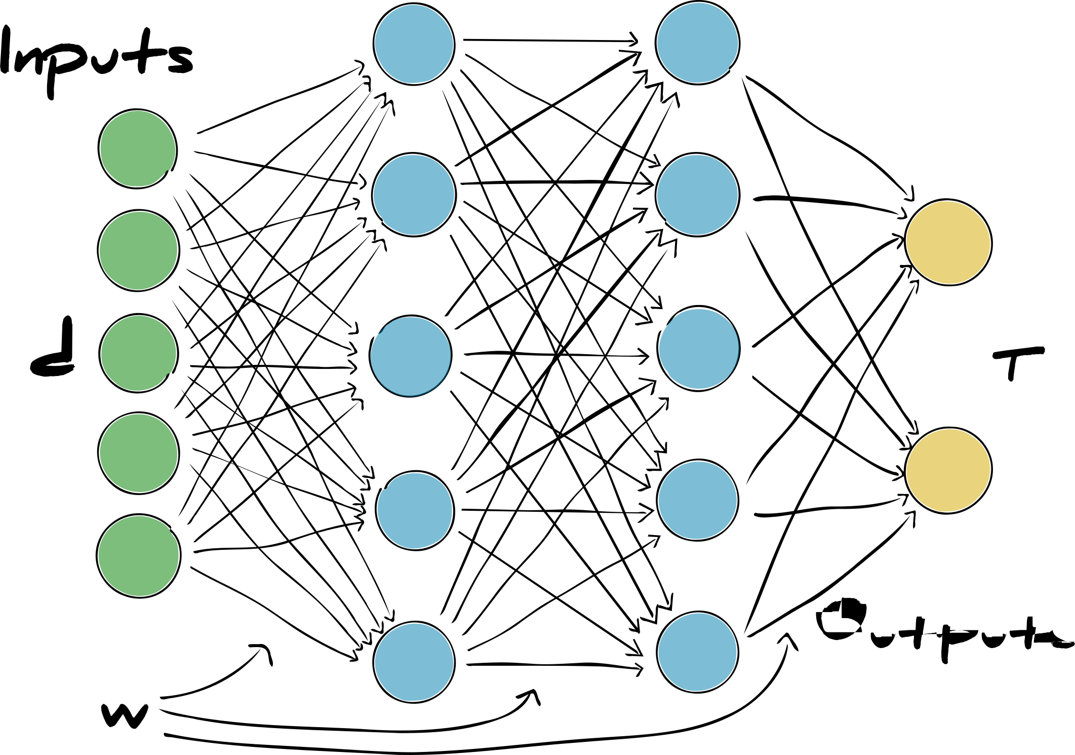
$$\mathbb{NN}(\boldsymbol{w},\boldsymbol{\alpha}) : {\bf d}\rightarrow\boldsymbol{\tau}$$

An approximation to a model, $\mathcal{M} : {\bf d}\rightarrow{\bf t}$

What are they used for?¶

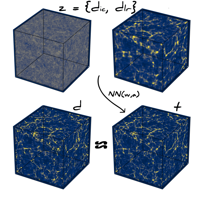
Emulation (generative networks)¶

$\mathbb{NN}(\boldsymbol{w},\boldsymbol{\alpha}) : {\bf z}\to{\bf t}$

${\bf t}\in\mathcal{P}({\bf t}|{\bf z})\simeq{\bf d}\in\mathcal{P}({\bf d})$

Classification¶

$\mathbb{NN}(\boldsymbol{w},\boldsymbol{\alpha}) : {\bf d}\to{\bf t}$

${\bf t}\in\mathcal{P}({\bf t})\simeq{\bf d}\in\mathcal{P}(\textrm{type}|{\bf d})$

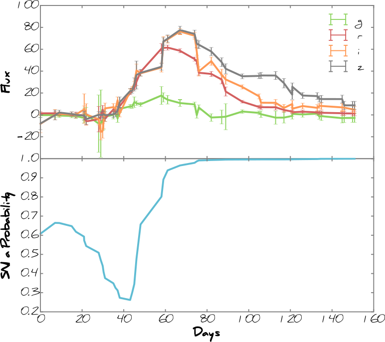
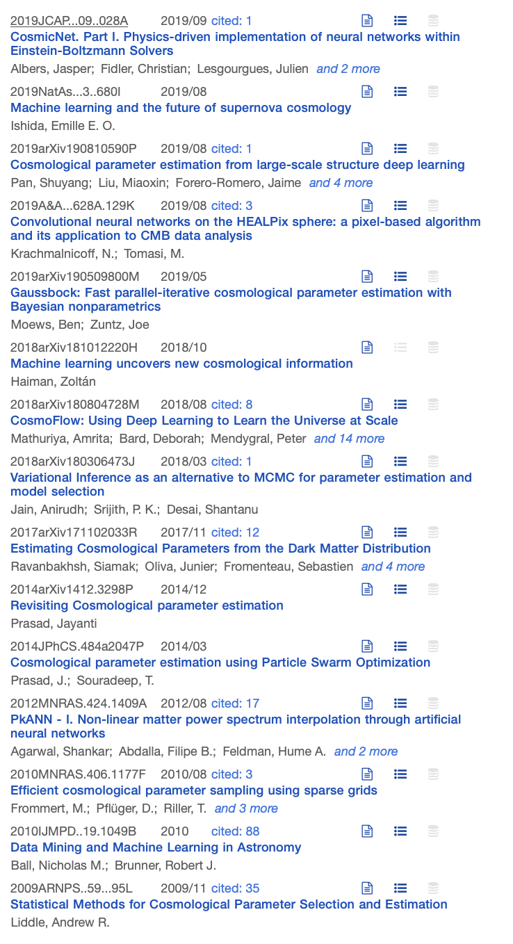
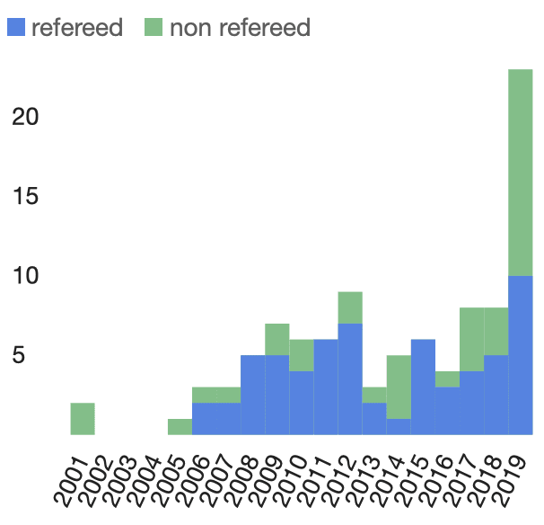
Extremely popular for cosmological parameter estimation¶

$\mathcal{M} : \boldsymbol{\theta}\to{\bf d}$
$\overset{~}{\mathbb{NN}}(\boldsymbol{w},\boldsymbol{\alpha}) : {\bf d}\to\hat{\boldsymbol{\theta}}$

Unfortunately...¶

None of these work in a scientifically rigourous way!¶

To see why we need to do some stats¶

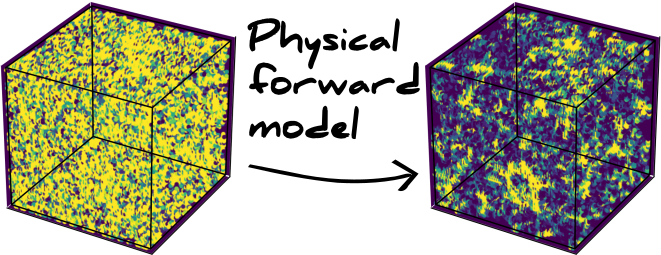
A physical model $\small\mathcal{M} : \boldsymbol{\theta}\to{\bf d}$¶

The generator of data $({\bf d})$ with parameters $(\boldsymbol{\theta})$

The likelihood and the posterior¶

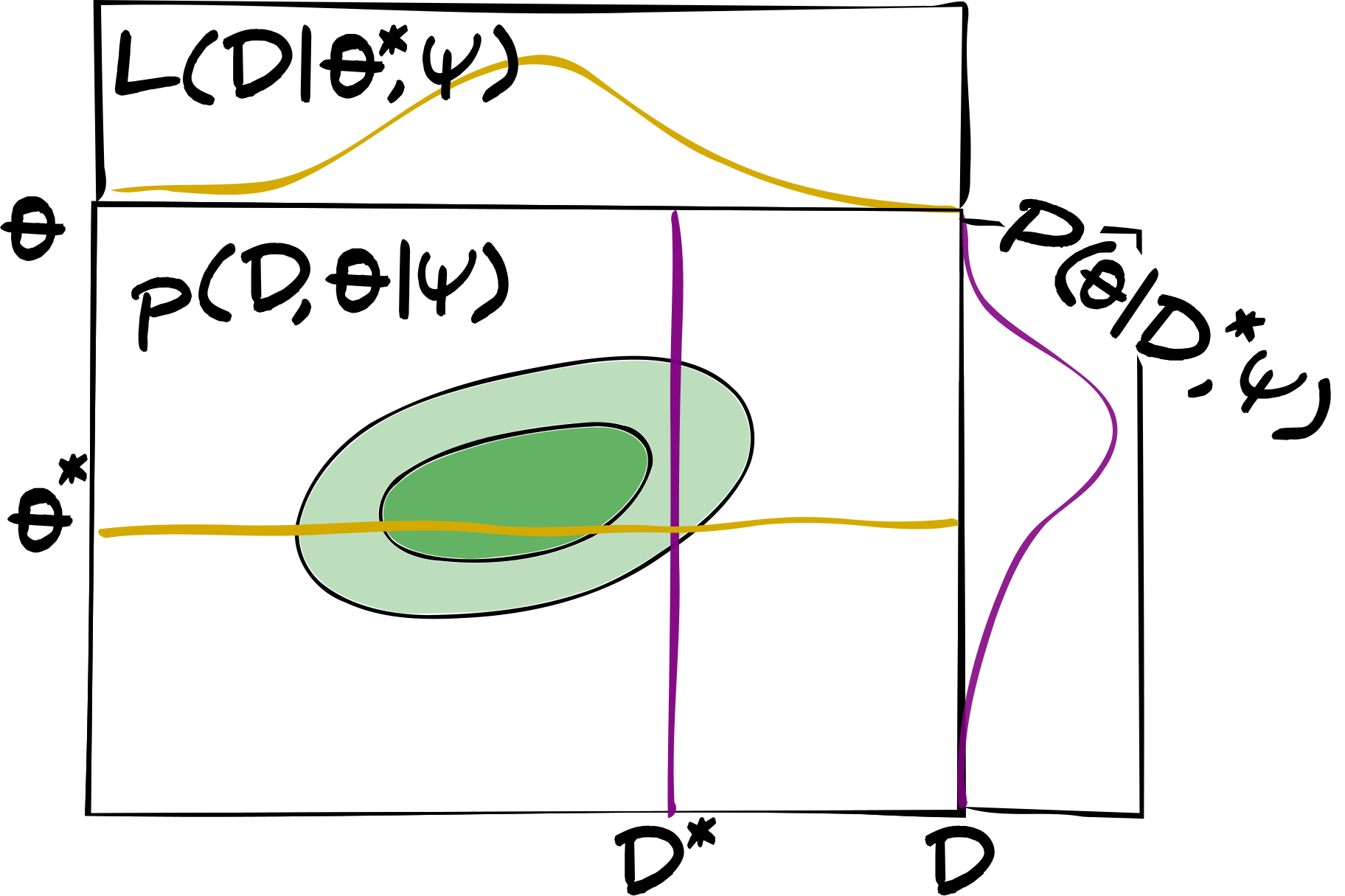
Likelihood $\mathcal{L}({\bf d}|\boldsymbol{\theta}^*)$
What is the probability that the model generates data ${\bf d}$ given a set of model parameters $\boldsymbol{\theta}^*$?

Posterior $\mathcal{P}(\boldsymbol{\theta}|{\bf d}^*)$
What is the probability that model parameters $\boldsymbol{\theta}$ generate the data ${\bf d}^*$?

Maximum likelihood estimates¶

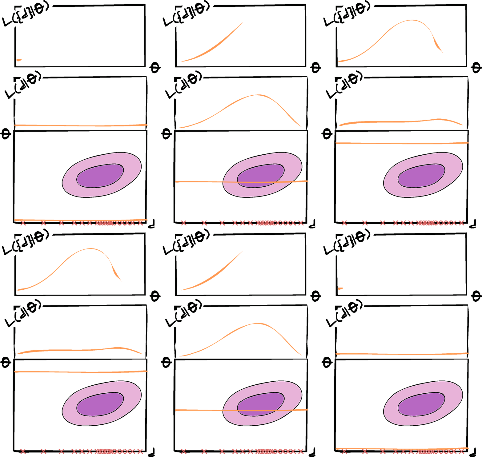
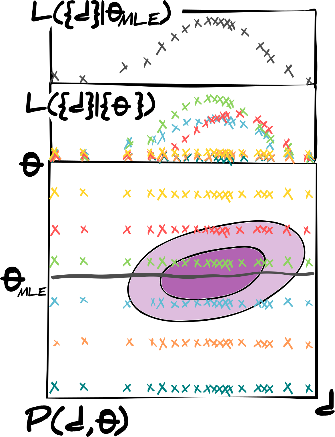Which value of the model parameters $\boldsymbol{\theta}$ is most likely to generate the observed population of data $\{{\bf d}\}$?

$$\mathcal{L}(\{{\bf d}\}|\boldsymbol{\theta}_\textsf{MLE})=\underset{\boldsymbol{\theta}\in\boldsymbol{\Theta}}{\textsf{Sup}}~\mathcal{L}(\{{\bf d}\}|\boldsymbol{\theta})$$

Training a network¶

$\mathcal{M} : {\bf d} \to {\bf t}$ approximator

$$\mathbb{NN}(\boldsymbol{w}, \boldsymbol{\alpha}) : {\bf d}\to\boldsymbol{\tau}$$
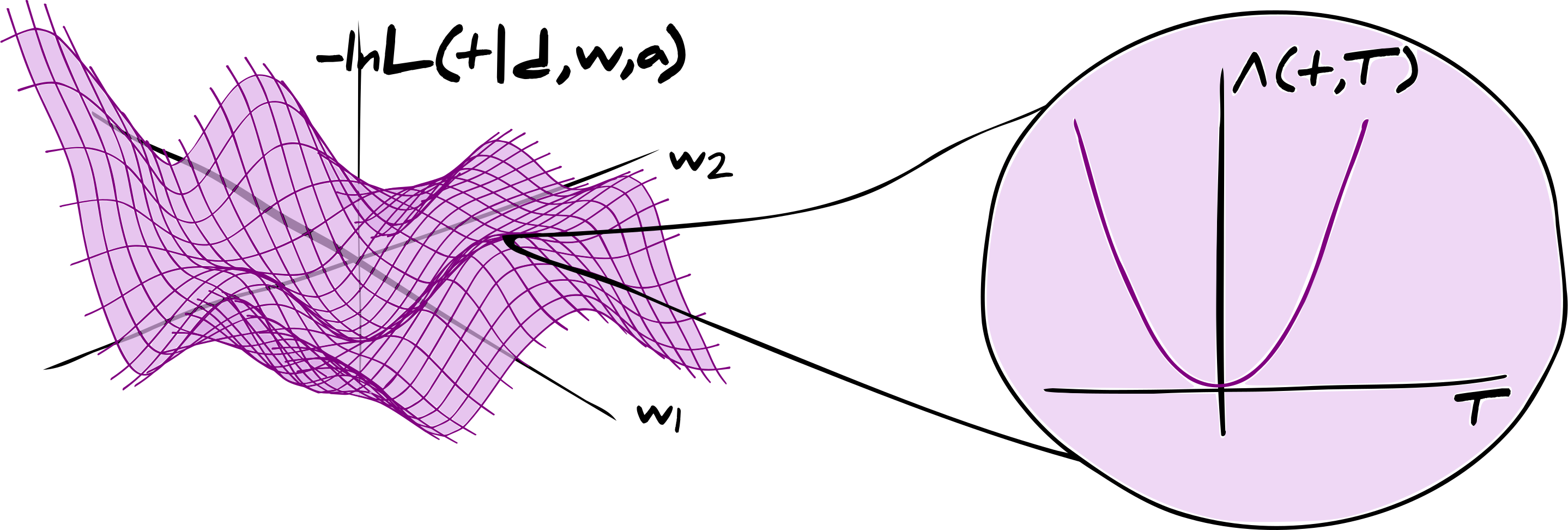
Cost function and likelihood $$\boldsymbol{\Lambda}({\bf t}, \boldsymbol{\tau}) = -\ln\mathcal{L}({\bf t}|{\bf d},\boldsymbol{w}^*,\boldsymbol{\alpha}^*)$$

$\boldsymbol{\Lambda}({\bf t},\boldsymbol{\tau})$
smooth and convex

$\mathcal{L}({\bf t}|{\bf d},\boldsymbol{w},\boldsymbol{\alpha})$
complex, discrete and possibly non-convex in $\boldsymbol{w}$ and $\boldsymbol{\alpha}$

Optimising a network¶

Given a set of training data $\{{\bf d}^\textrm{train}_i, {\bf t}^\textrm{train}_i|i\in[1,n_\textrm{train}]\}$ what is the maximum likelihood estimate of the weights?

$$\small\boldsymbol{w}^\textrm{MLE}=\underset{\boldsymbol{w}}{\textrm{argmax}}\left[\mathcal{L}(\{{\bf t}^\textrm{train}_i|i\in[1, n_\textrm{train}]\}|\{{\bf d}^\textrm{train}_i|i\in[1, n_\textrm{train}]\}, \boldsymbol{w}, \boldsymbol{\alpha}^*)\right]$$

Where the problem starts¶

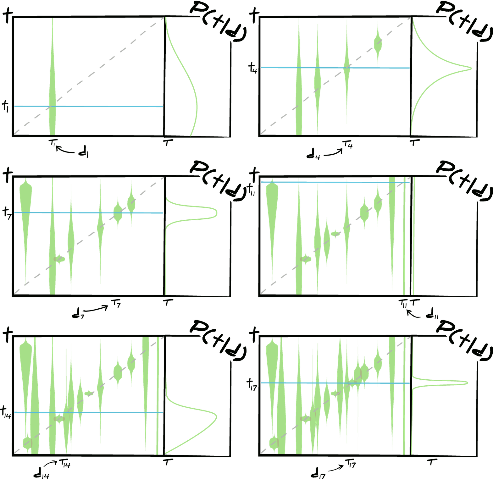
The posterior predictive density $\mathcal{P}({\bf t}|{\bf d})$¶

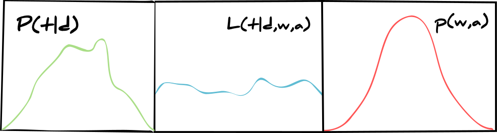
$$\mathcal{P}({\bf t}|{\bf d})= \int d\boldsymbol{w}\boldsymbol{\alpha}\mathcal{L}({\bf t}|{\bf d},\boldsymbol{w},\boldsymbol{\alpha})p(\boldsymbol{w},\boldsymbol{\alpha})$$

Failure of traditional networks¶

$p(\boldsymbol{w}, \boldsymbol{\alpha})=\delta(\boldsymbol{w}-\boldsymbol{w}^\textrm{local MLE}, \boldsymbol{\alpha}-\boldsymbol{\alpha}^*)$

$\mathcal{P}({\bf t}|{\bf d}) =\delta(\boldsymbol{\tau})$

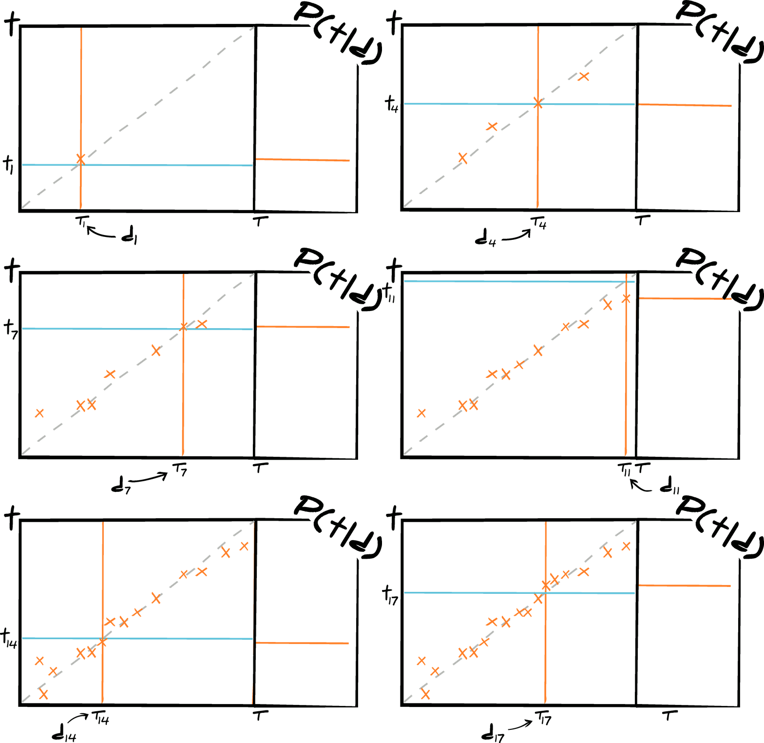
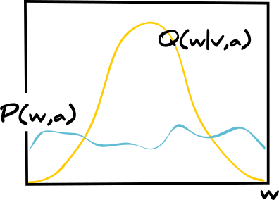
Variational inference¶

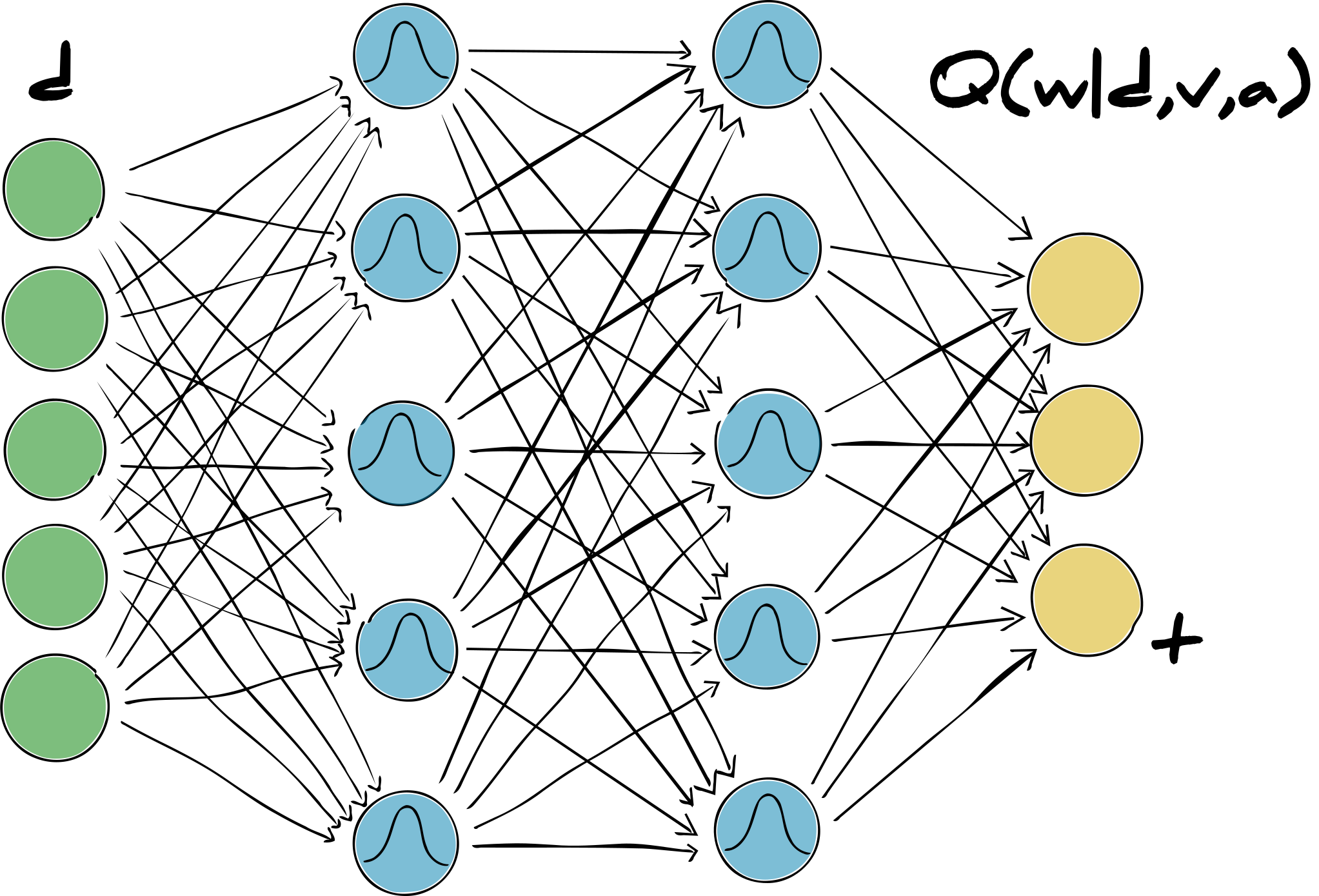
$$\tiny\mathcal{P}({\bf t}|{\bf d})=\int d\boldsymbol{w}d\boldsymbol{v}d\boldsymbol{\alpha}~\mathcal{L}({\bf t}|{\bf d},\boldsymbol{w},\boldsymbol{\alpha})\mathcal{Q}(\boldsymbol{w}|\boldsymbol{v}, \boldsymbol{\alpha}, \{{\bf d}^\textrm{train}_i, {\bf t}^\textrm{train}_i|i\in[1, n_\textrm{train}]\})p(\boldsymbol{v},\boldsymbol{\alpha})$$

Still depends on training the complex likelihood surface and choice of variational distribution¶

$$\begin{align*}\tiny \mathcal{P}({\bf t}|{\bf d})&=\tiny\int d\boldsymbol{w}d\boldsymbol{v}d\boldsymbol{\alpha}~\mathcal{L}({\bf t}|{\bf d},\boldsymbol{w},\boldsymbol{\alpha})\mathcal{Q}(\boldsymbol{w}|\boldsymbol{v}, \boldsymbol{\alpha}, \{{\bf d}^\textrm{train}_i, {\bf t}^\textrm{train}_i|i\in[1, n_\textrm{train}]\})\\ &\tiny\phantom{=hello}\times\delta(\boldsymbol{v}-\boldsymbol{v}^\textrm{local MLE}, \boldsymbol{\alpha}-\boldsymbol{\alpha}^*)\\ &\tiny=\int d\boldsymbol{w}~\mathcal{L}({\bf t}|{\bf d},\boldsymbol{w}, \boldsymbol{\alpha}^*)\mathcal{Q}(\boldsymbol{w}|\boldsymbol{v}^\textrm{local MLE}, \boldsymbol{\alpha}^*, \{{\bf d}^\textrm{train}_i, {\bf t}^\textrm{train}_i|i\in[1, n_\textrm{train}]\}). \end{align*}$$

Bayesian neural networks¶

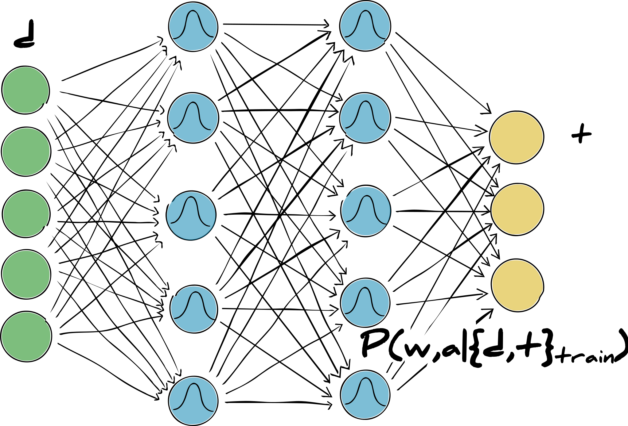
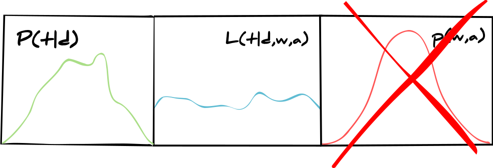
$$\begin{align*} \tiny \mathcal{P}({\bf t}|{\bf d}) =&\tiny~\int d\boldsymbol{w}d\boldsymbol{\alpha}~\mathcal{L}({\bf t}|{\bf d}, \boldsymbol{w}, \boldsymbol{\alpha})\mathcal{P}(\boldsymbol{w},\boldsymbol{\alpha}|\{{\bf d}^\textrm{train}_i, {\bf t}^\textrm{train}_i|i\in[1, n_\textrm{train}]\})\\ \tiny =&\tiny~\int d\boldsymbol{w}d\boldsymbol{\alpha}~\mathcal{L}({\bf t}|{\bf d}, \boldsymbol{w}, \boldsymbol{\alpha})\prod_i^{n_\textrm{train}}\mathcal{L}({\bf t}^\textrm{train}_i|{\bf d}^\textrm{train}_i,\boldsymbol{w},\boldsymbol{\alpha})p(\boldsymbol{w},\boldsymbol{\alpha}). \end{align*} $$

Still dependent on the training data!¶

Classical network : $\tiny p(\boldsymbol{w},\boldsymbol{\alpha}) = \delta(\boldsymbol{w}-\boldsymbol{w}^\textrm{MLE},\boldsymbol{\alpha}-\boldsymbol{\alpha}^*)$

Variational inference : $\tiny p(\boldsymbol{w},\boldsymbol{\alpha}) = \mathcal{Q}(\boldsymbol{w}|\boldsymbol{v}^\textrm{local MLE}, \boldsymbol{\alpha}^*, \{{\bf d}^\textrm{train}_i, {\bf t}^\textrm{train}_i|i\in[1, n_\textrm{train}]\})$

Bayesian neural networks : $\tiny p(\boldsymbol{w},\boldsymbol{\alpha}) =\prod_i^{n_\textrm{train}}\mathcal{L}({\bf t}^\textrm{train}_i|{\bf d}^\textrm{train}_i,\boldsymbol{w},\boldsymbol{\alpha})p(\boldsymbol{w},\boldsymbol{\alpha})$

How can we use a neural network then?¶

Build it into the physical model¶

Method 1 : Model extension¶

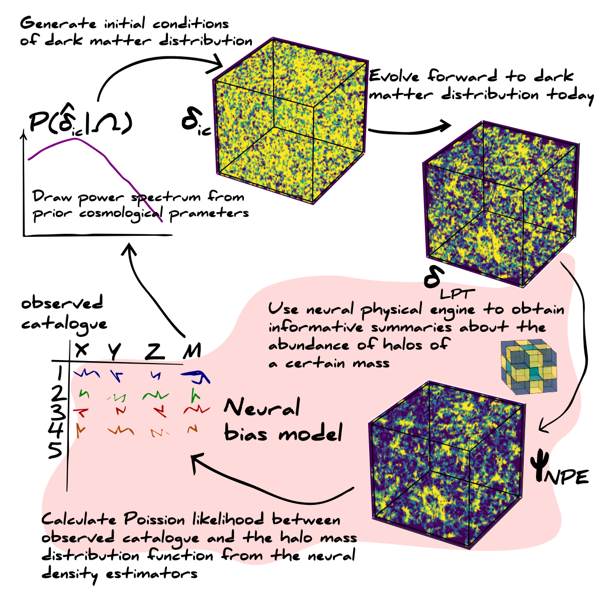
We infer the neural network¶

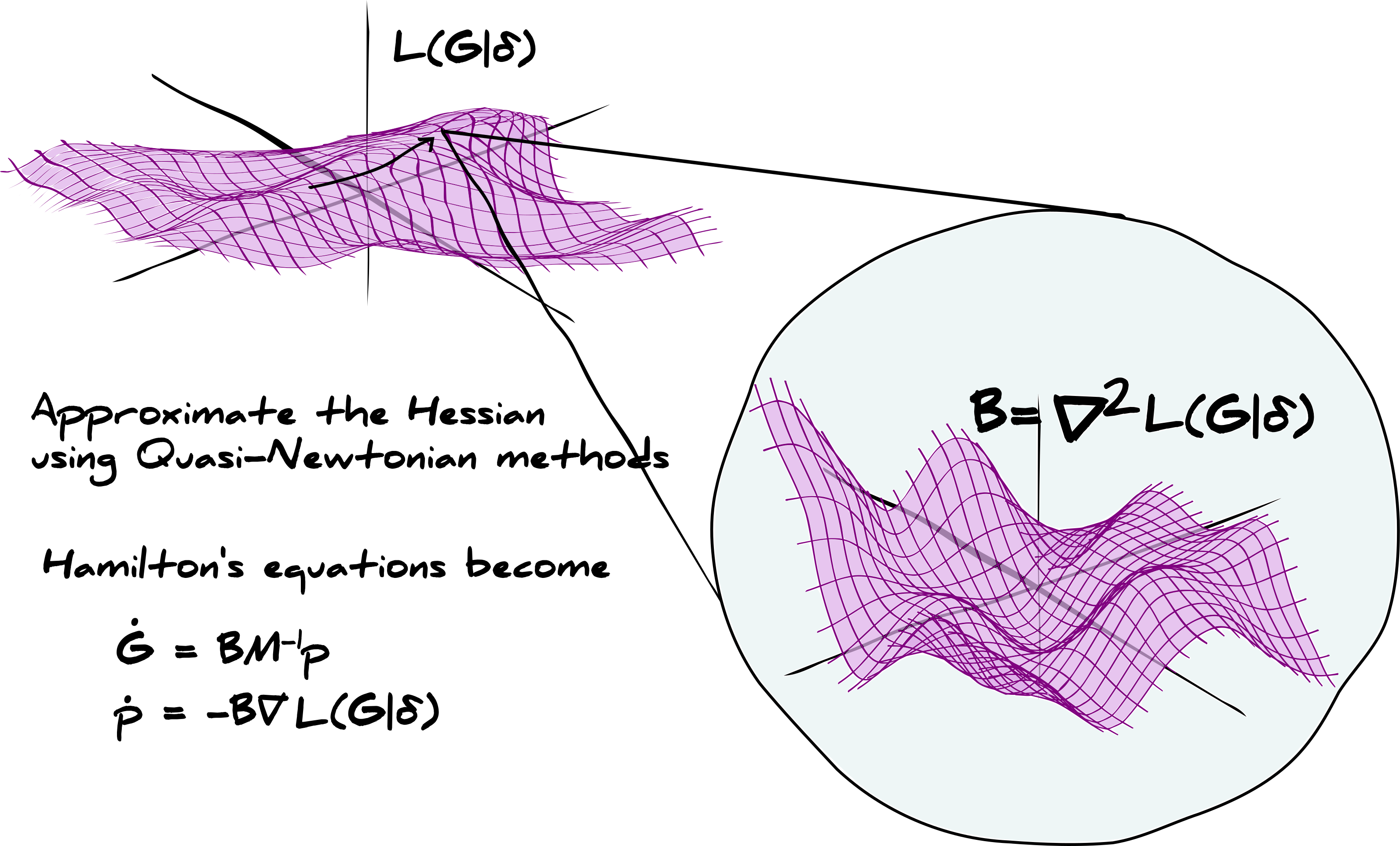
HMCLET¶

Hamiltonian Monte Carlo¶

_{Introduce momentum ${\small {\bf p}\leftarrow\mathcal{N}({\bf 0},{\bf M})}$ and solve Hamilton's equations}

$$\begin{align*} {\Tiny\mathcal{H}(\boldsymbol{\theta}, {\bf p}) }&{\Tiny~= \mathcal{V}(\boldsymbol{\theta}) + \mathcal{K}({\bf p})}\\ &{\Tiny~=\mathcal{L}(\boldsymbol{\theta}|\boldsymbol{\delta})-\log\left[\pi(\boldsymbol{\theta})\right]+\frac{1}{2}{\bf p}^T{\bf M}^{-1}{\bf p}} \end{align*}$$ _{Accept samples according to probability} $$\begin{equation*} {\Tiny\alpha = \textrm{Min}\left[\exp\left(\Delta\mathcal{H}\right), 1\right]} \end{equation*}$$

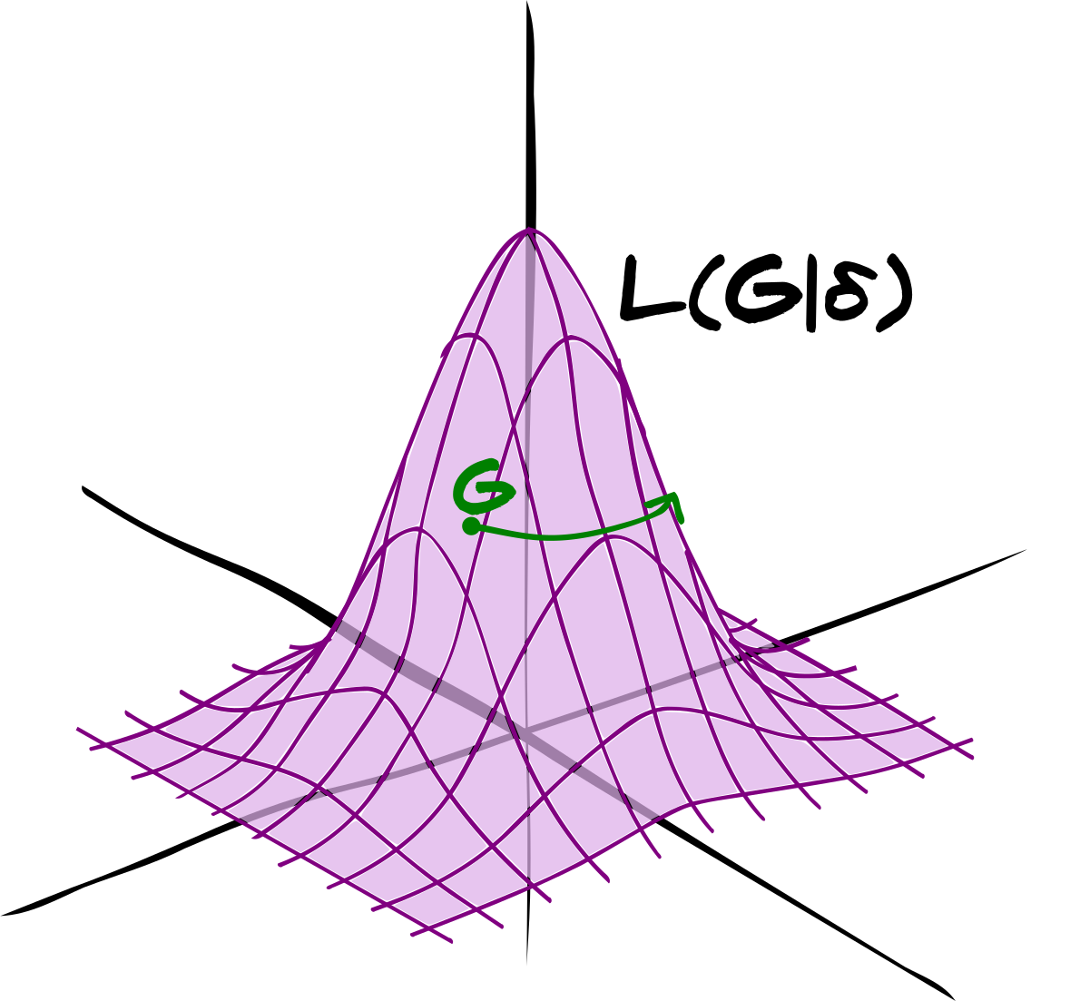
Evolve using ${\Tiny\dot{\boldsymbol{\theta}}= {\bf M}^{-1}{\bf p}}$ and ${\Tiny\dot{\bf p}= -\nabla\mathcal{V}(\boldsymbol{\theta})}$

Use second order geometric information¶

Neural physical engines¶

Build networks using physical principles.

Reduces number of parameters
Increases computational efficiency
Decreases overfitting
Improves interpretability

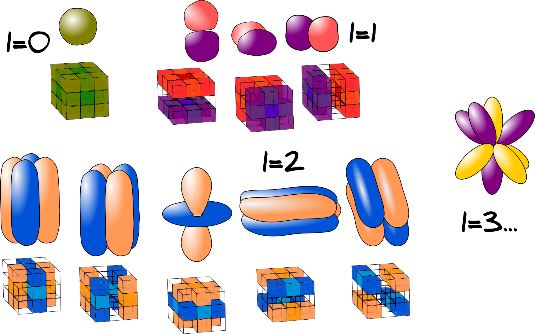
Convolutions for translational invariance¶

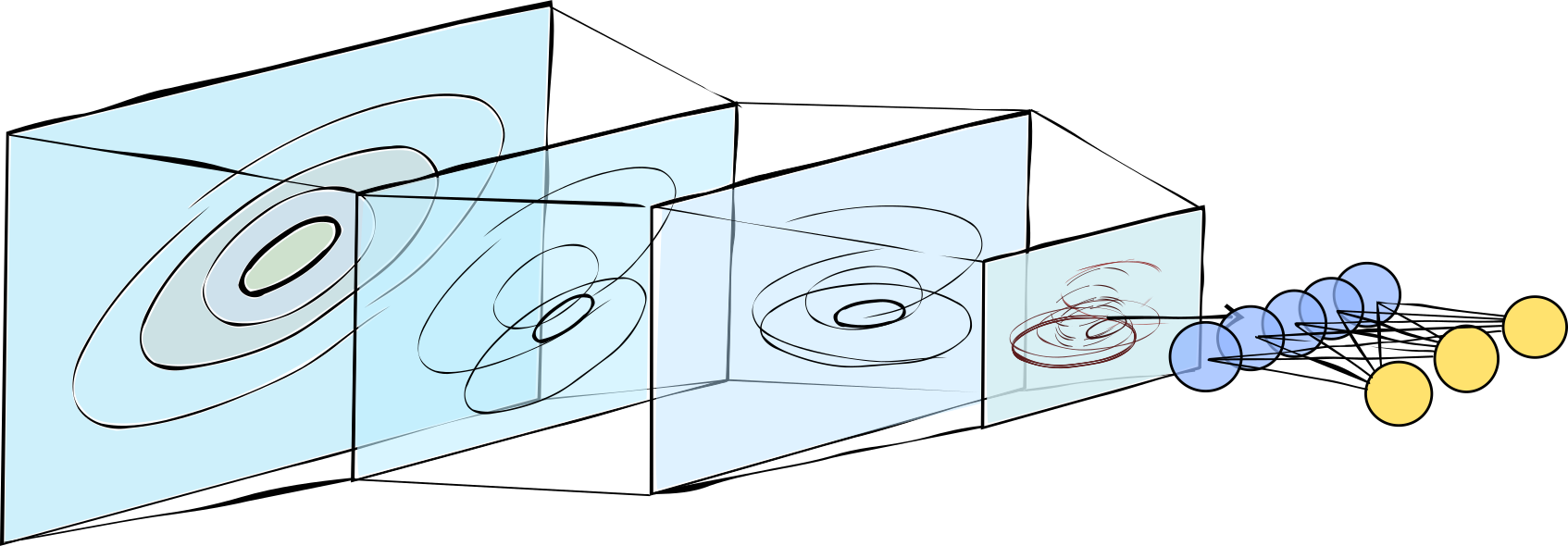
Use only causally relevant features¶

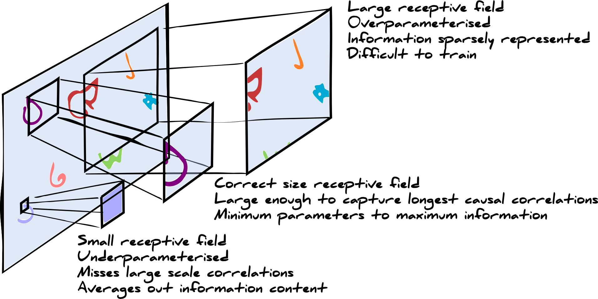
Use only informative features¶

_{github:multipole_kernels}

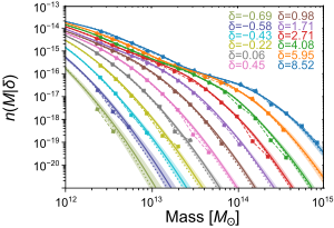
Halo mass distribution function¶

Neural density estimators¶

Halo mass distribution function is a smooth function of mass given a density environment¶

Use a mixture density network¶

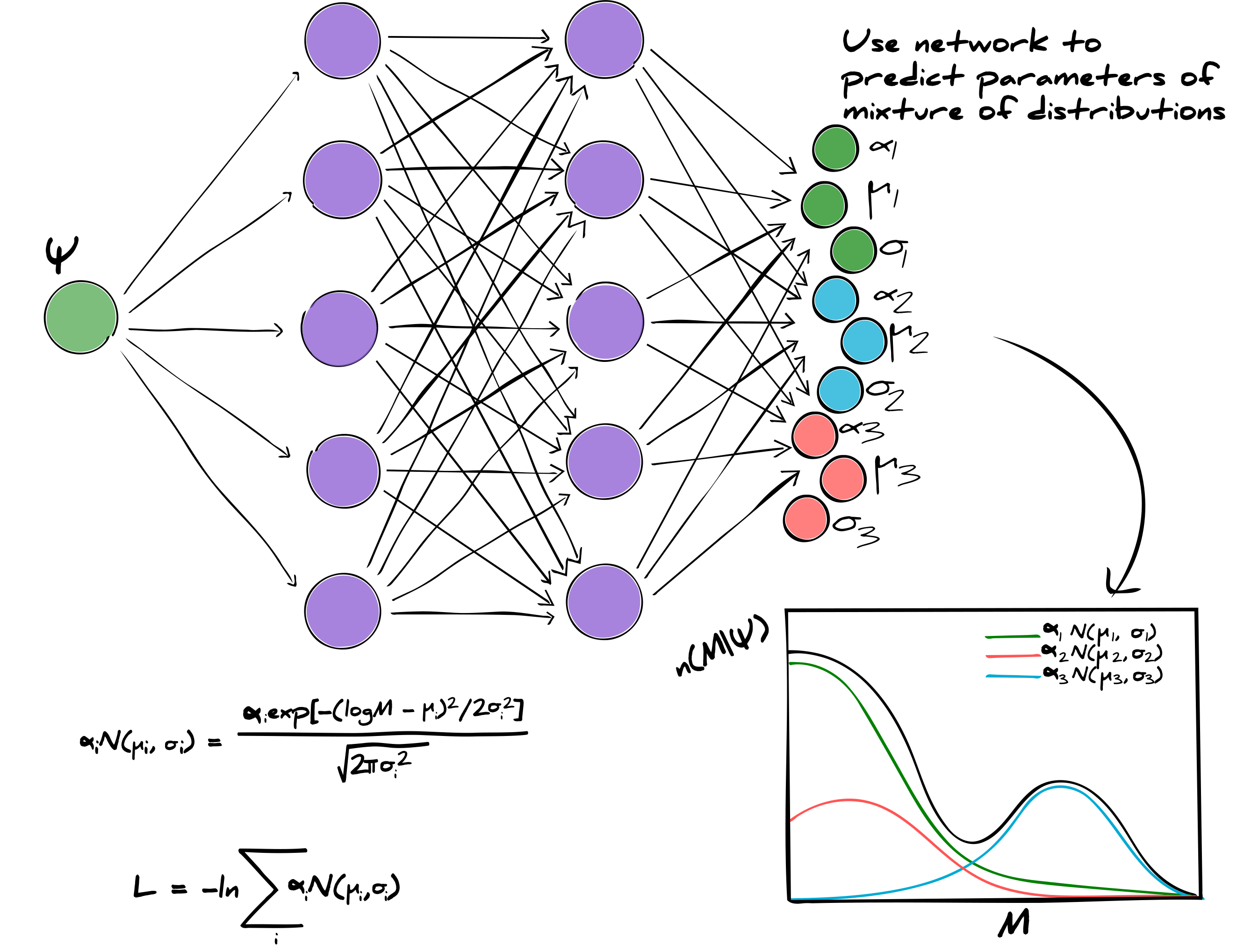
Our neural density estimator¶

$$\begin{align*} {\tiny n(M|\delta) =}&{\tiny \sum_i^N\alpha(\boldsymbol{\psi}, \boldsymbol{\theta}_i^{\boldsymbol{\alpha}})\mathcal{N}\left(\mu(\boldsymbol{\psi}, \boldsymbol{\theta}_i^{\boldsymbol{\mu}}), \sigma(\boldsymbol{\psi}, \boldsymbol{\theta}_i^{\boldsymbol{\sigma}})|M\right),}\\ {\tiny =}&{\tiny \sum_i^N\frac{\alpha(\boldsymbol{\psi}, \boldsymbol{\theta}_i^{\boldsymbol{\alpha}})}{\sqrt{2\pi\left(\sigma(\boldsymbol{\psi}, \boldsymbol{\theta}_i^{\boldsymbol{\sigma}})\right)^2}}\exp\left[-\frac{\left(\log(M) - \mu(\boldsymbol{\psi}, \boldsymbol{\theta}_i^{\boldsymbol{\mu}})\right)^2}{2\left(\sigma(\boldsymbol{\psi}, \boldsymbol{\theta}_i^{\boldsymbol{\sigma}})\right)^2}\right],}\end{align*} $$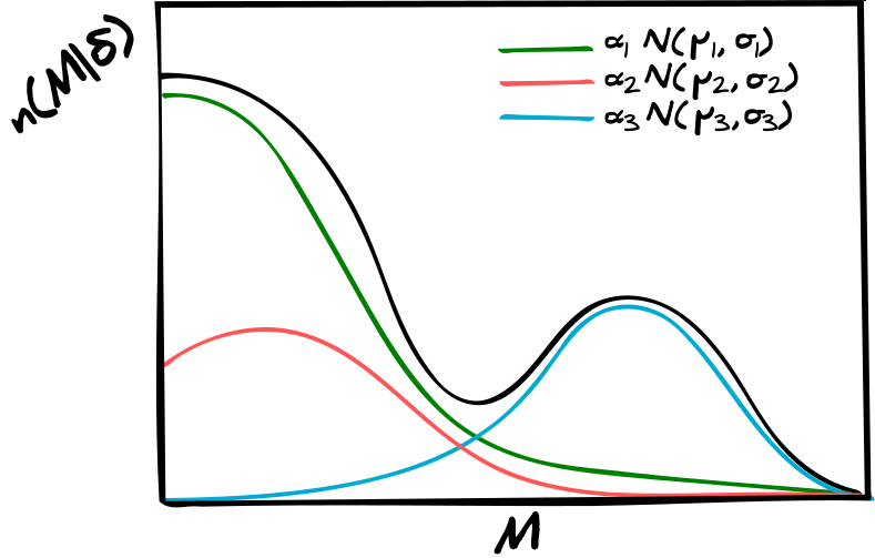

$$ \begin{align*} {\tiny\alpha_i} & {\tiny=\text{softplus}(w_{i}^\alpha\boldsymbol{\psi}+b^\alpha_i),}\\ {\tiny\mu_i }&{\tiny = \left\{\begin{array}{ll} w_{i}^\mu\boldsymbol{\psi}+b^\mu_i&i=0\\ \textrm{Max}\left[0,~ w_{i}^\mu\boldsymbol{\psi}+b^\mu_i\right]+\mu_{i-1}&i>0\\ \end{array}\right.,}\\ {\tiny\sigma_i} &{\tiny = \text{softplus}(w_{i}^\sigma\boldsymbol{\psi}+b^\sigma_i)\;,} \end{align*} $$

_{2 Gaussians with
${\Tiny\boldsymbol{b}^\alpha \to \boldsymbol{b}^\alpha +\log(10^{-3})}$, ${\Tiny b_0^\mu \to b_0^\mu + \log\left(2\times10^{12}\right)}$ and ${\Tiny\boldsymbol{b}^\sigma\to \boldsymbol{b}^\alpha + \log(10^3)}$.}

Likelihood¶

$$\begin{align*} {\Tiny\mathcal{L} =}&{\Tiny \sum_{j\in\textrm{catalogue}}\log\left[\sum_i^N\frac{\alpha_{i,j}}{\sqrt{2\pi\sigma_{i,j}^2}}\exp\left[-\frac{\left(\log(M_j) - \mu_{i,j}\right)^2}{2\sigma_{i,j}^2}\right]\right]}\\ &{\Tiny - V\sum_{j\in\textrm{voxels},i=1}^N\frac{\alpha_{i,j}}{2}\exp\left[\frac{\sigma_{i,j}^2}{2}\right]\textrm{erfc}\left[\frac{\log\left(M_\textrm{th}\right) - \mu_{i,j} - \sigma_{i,j}^2}{\sqrt{2\sigma_{i,j}^2}}\right].} \end{align*}$$

Sample the power spectrum¶

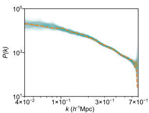✓ Power spectra remain smooth and close to prior

Sample the weights of the neural bias model¶

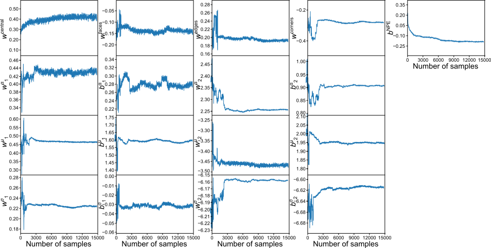
✓ Weight values are properly sampled after burn in
✓ NPE acts as a contrast enhancer

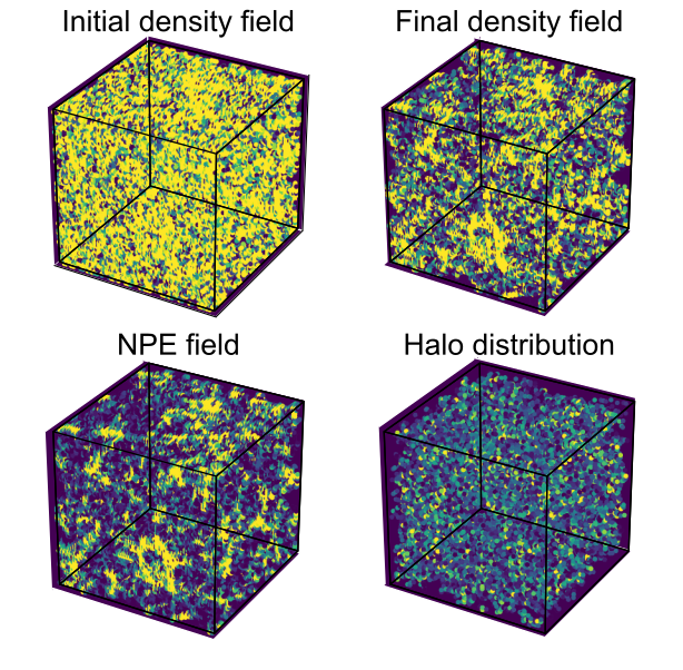
See the effects of the neural physical engine¶

✓ Non-local information is used to improve fit

And what does the halo mass distribution function look like?¶

Halo mass distribution function from neural bias model¶

✓ Fits data!

Method 2 : Likelihood-free inference¶

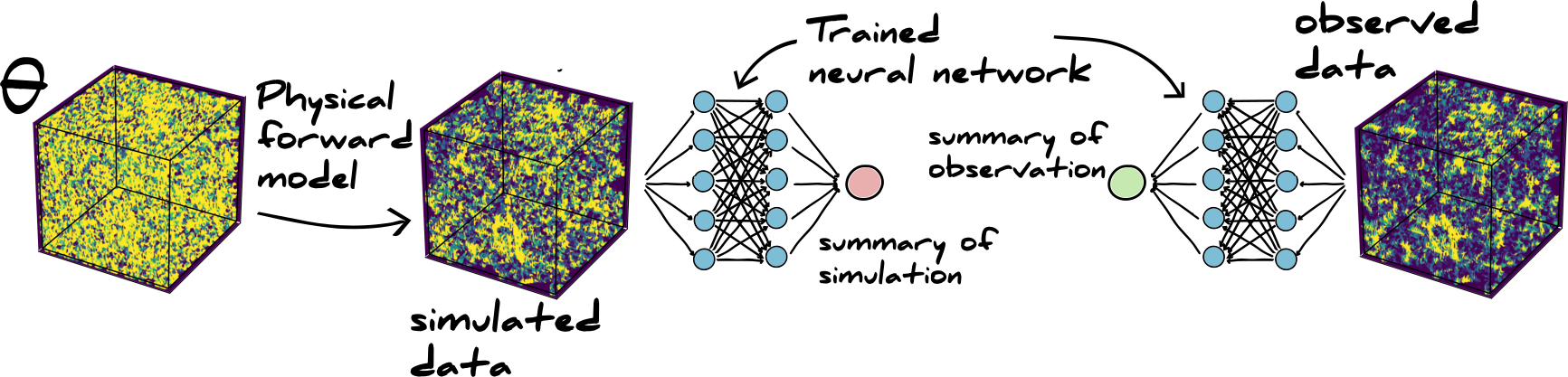
Likelihood-free inference using machine learning¶

Approximate Bayesian computation¶

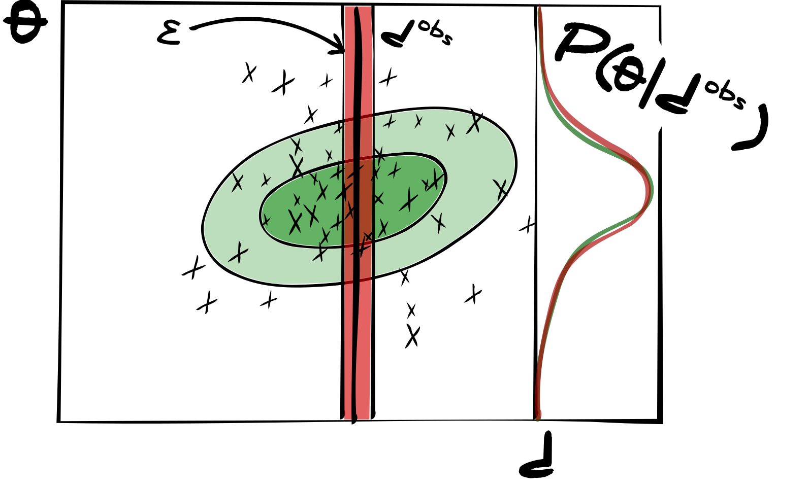
Why even introduce the neural network?¶

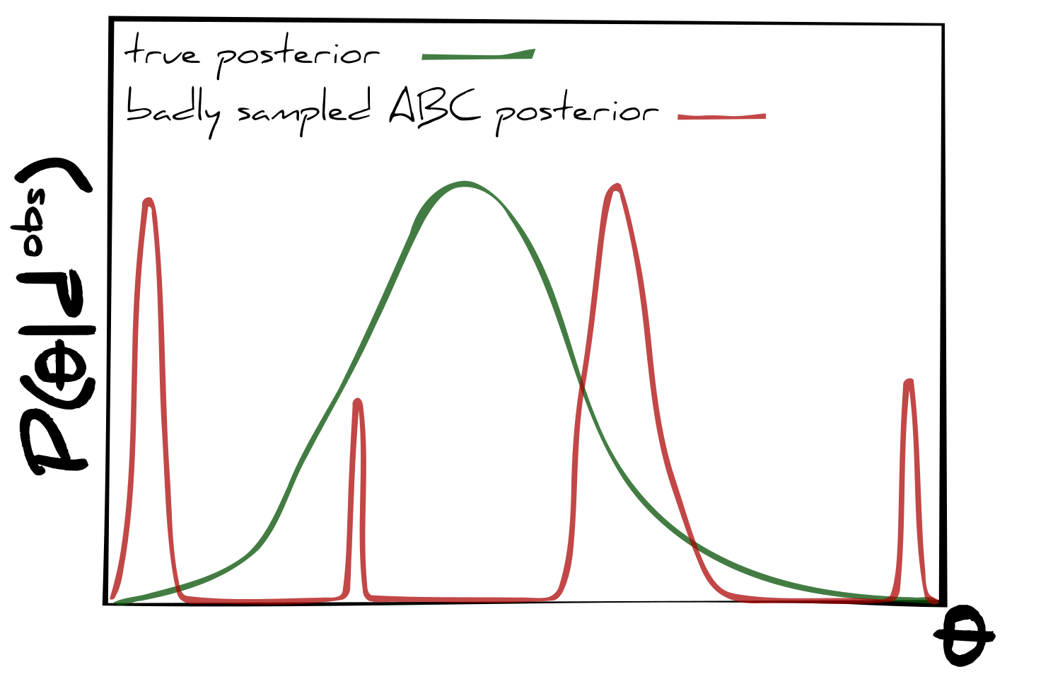
Inadequate sampling¶

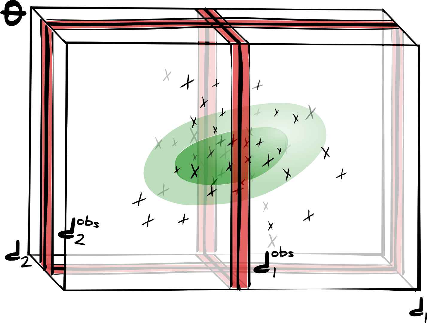
Impossibly large numbers of simulations become necessary to correctly sample the posterior

We need to do some compression¶

Any pretrained neural network could be used¶

Is there a well motivated choice?¶

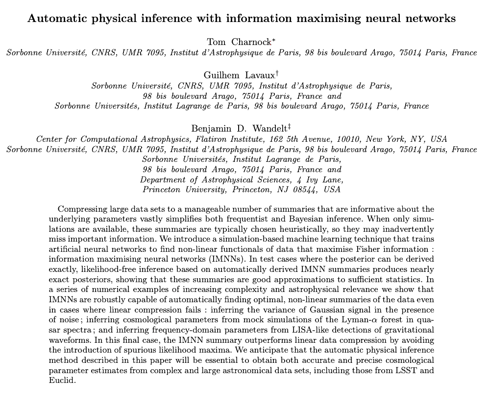
Information maximising neural networks¶

Which function $\mathscr{f}: \mathbb{R}^{\bf d}\to \mathbb{R}^\boldsymbol{\theta}$ maximises the Fisher information of the summaries ${\bf x}$ from that function?

$$\mathcal{L}({\bf d}|\boldsymbol{\theta})\to\mathcal{L}({\bf x}|\boldsymbol{\theta}, {\bf d})$$

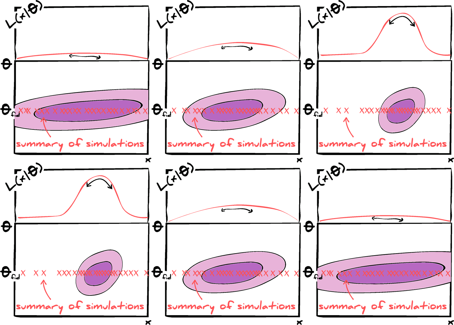
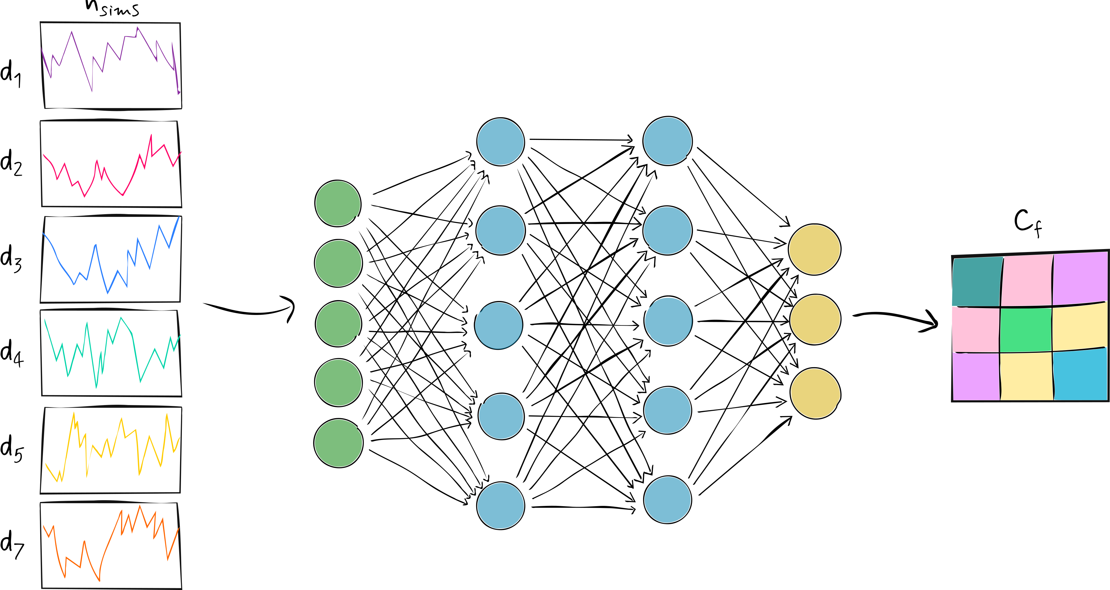
Fisher information of the network summaries¶

Simulations $\{{\bf d}_i|i\in[1, n_{\bf d}]\}$ at a single parameter value $\boldsymbol{\theta}^*$¶

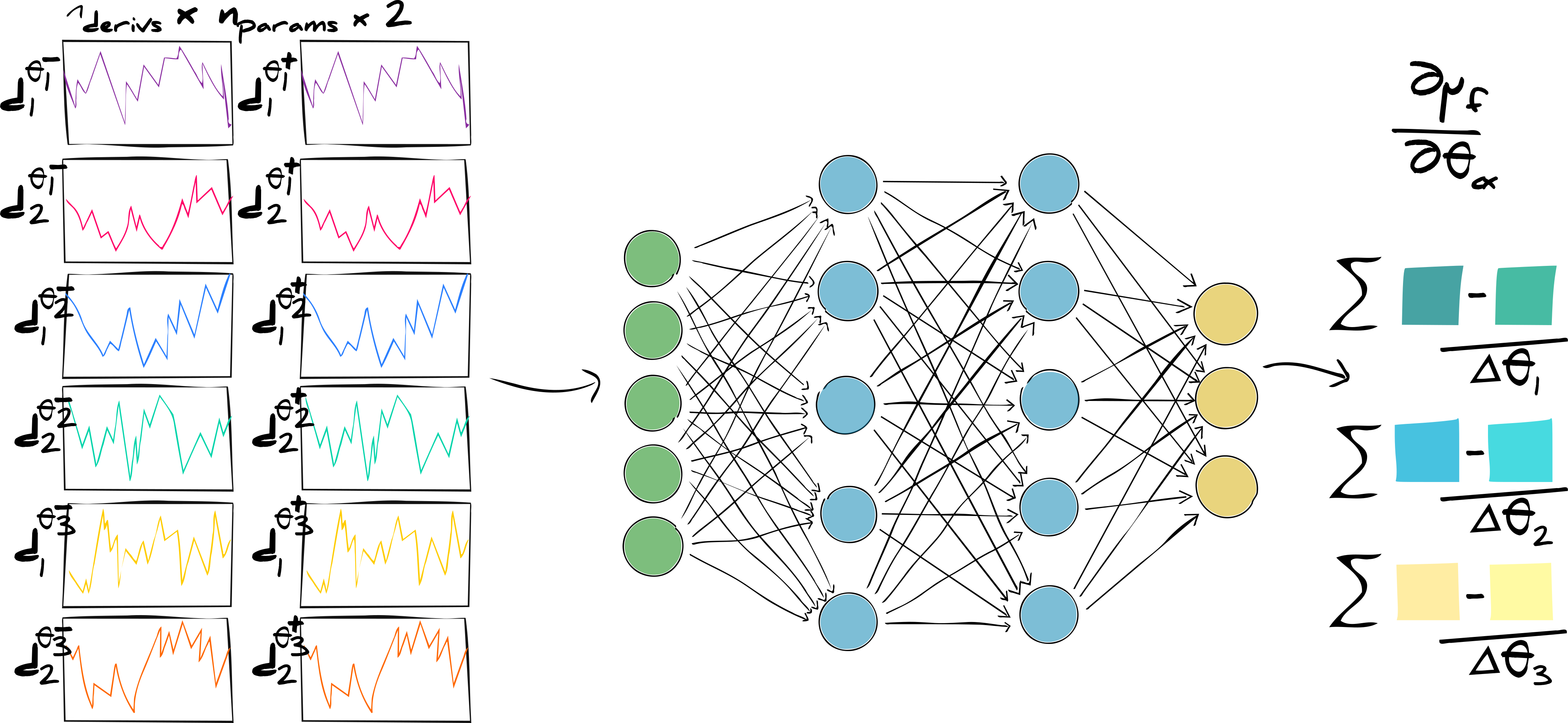
Seed matched simulations $\{{\bf d}_i^{\pm}|i\in[1, n_{\bf p}]\}$ at perturbed fiducial paremeters $\Delta\boldsymbol{\theta}^\pm=\boldsymbol{\theta}\pm\boldsymbol{\delta}$¶

Calculate the covariance¶

Calculate the derivative of the mean of the summaries with respect to the parameters¶

Calculate the Fisher information¶

$${\bf F}_{\alpha\beta}=\frac{\partial\mu_\mathscr{f}}{\partial\theta_\alpha}^T{\bf C}^{-1}_\mathscr{f}\frac{\partial\mu_\mathscr{f}}{\partial\theta_\beta}$$

This Gaussian form forces the summaries to be Gaussianised

Optimise the tunable parameters of the network such that $\ln|{\bf F}_{\alpha\beta}|$ is maximised!¶

Once converged the network compresses and Gaussianises the data without losing information*¶

*in the optimal case...

And we get free maximum likelihood estimates...¶

$$\boldsymbol{\theta}^\textsf{MLE}_\alpha=\boldsymbol{\theta}_\alpha^*+{\bf F}_{\alpha\beta}^{-1}{\bf C}_\mathscr{f}^{-1}\frac{\partial\mu_\mathscr{f}}{\partial\theta_\beta}({\bf x}-\mu_\mathscr{f})$$

And we can get free approximations of the posterior¶

$$\textsf{Cov}[\boldsymbol{\theta}_\alpha^\textsf{MLE},\boldsymbol{\theta}_\beta^\textsf{MLE}] \ge {\bf F}_{\alpha\beta}^{-1}$$

Or do likelihood-free inference¶

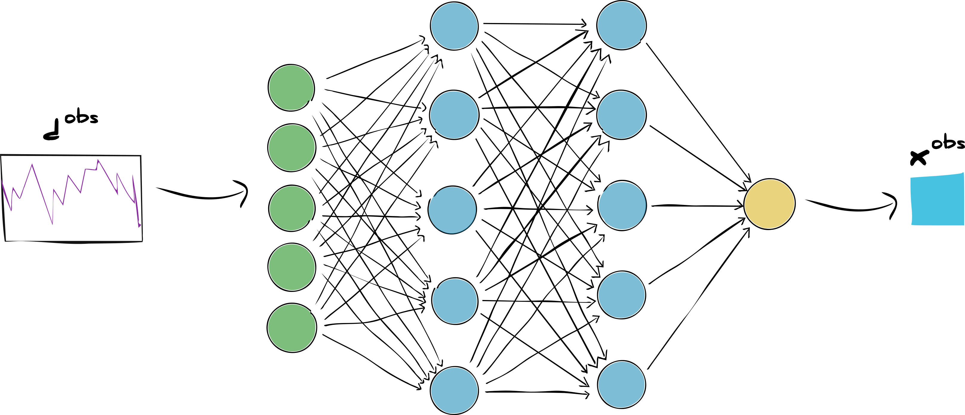
We pass our observed data through the network
(put it to the side)

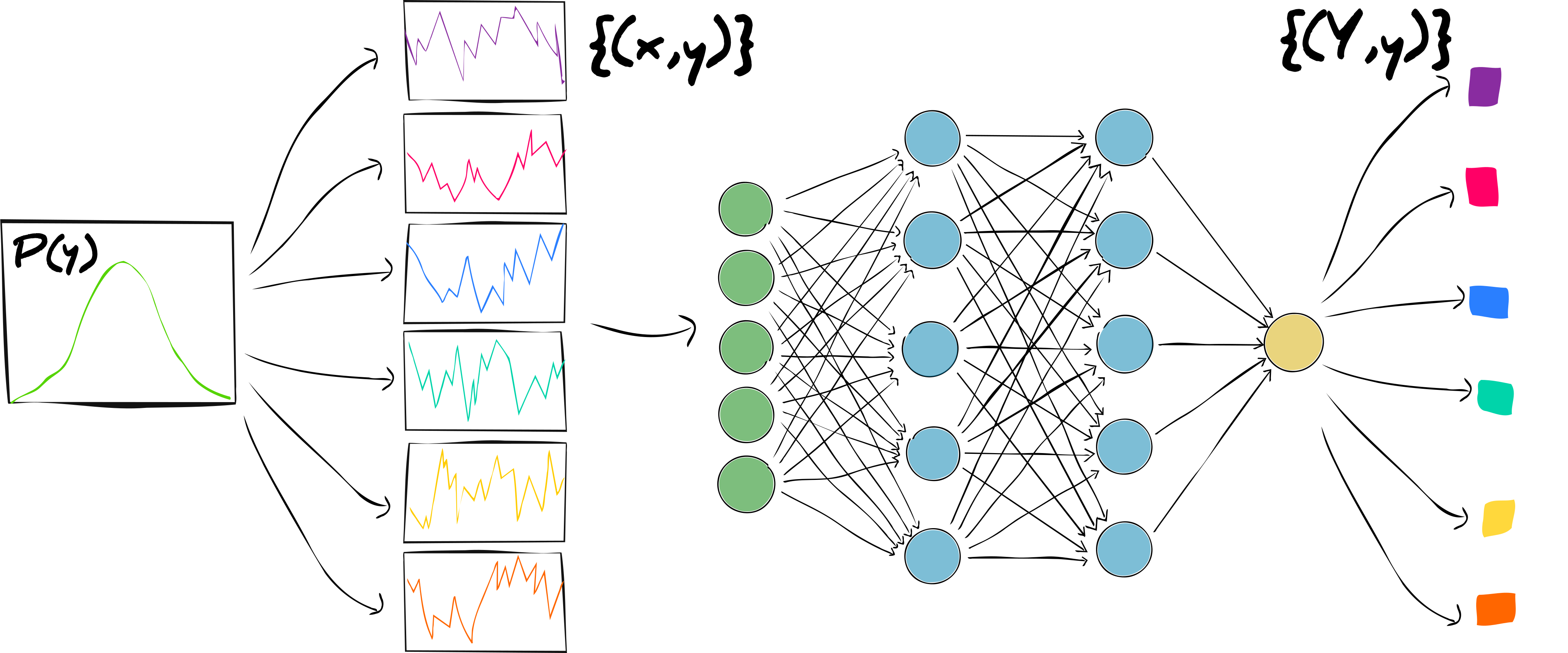
Draw simulations (cleverly?) from the prior model parameters, $\mathcal{P}(\boldsymbol{\theta})$ and pass them through the network¶

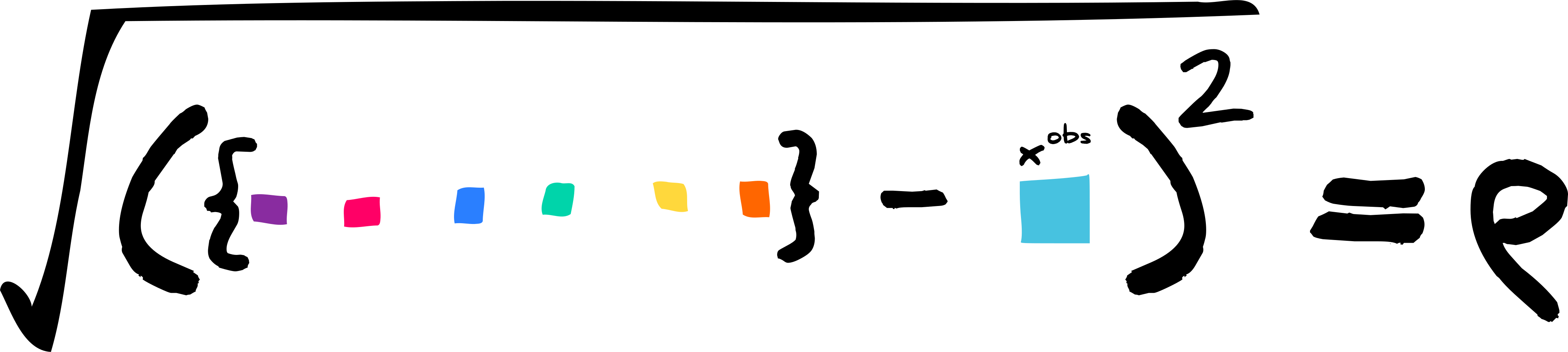
Measure the difference between the summarised simulations and the observed summary¶

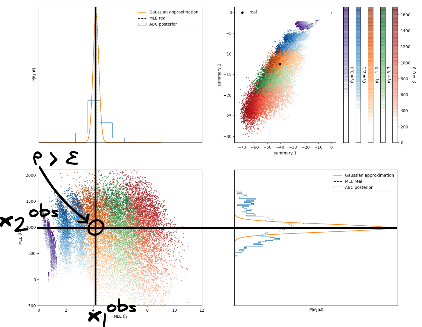
Compare distance between observed summaries and simulation summaries and select results within $\epsilon$

Conclusions¶

Neural networks are not to be trusted¶

They can make trusty companions - when the correct framework is introduced¶

Using statistics we can build them into the forward model to give us lossless summaries¶

Take home message¶

Stop doing machine learning, think, then start doing machine learning again!