Machine learning, statistics and the relation between
neural networks and physics
Tom Charnock
Institut d'Astrophysique de Paris
Slides available at presentations.charnock.fr/MLxPhysics




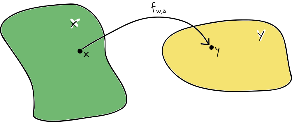
Neural networks - parameterisable functions $\mathscr{f}_{w,a}:x\in\mathcal{X}\mapsto y\in\mathcal{Y}$
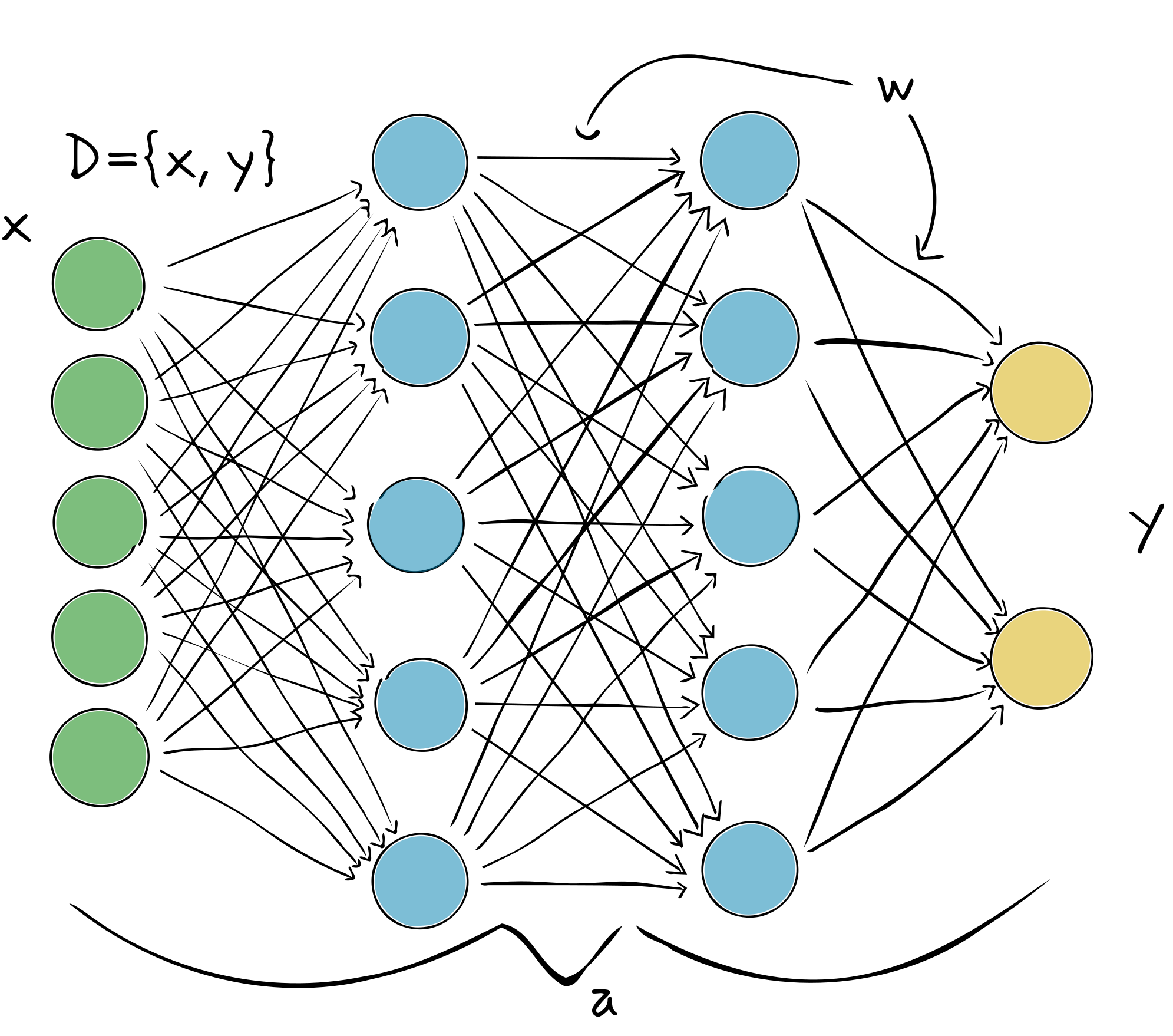
Stacks of non-linear activated weighted sums - \\(\displaystyle n_j^l = \phi\left(\sum_iw_{ji}n^{l-1}_i+b_j\right)\\)
Network architectures (actually doing different physics)
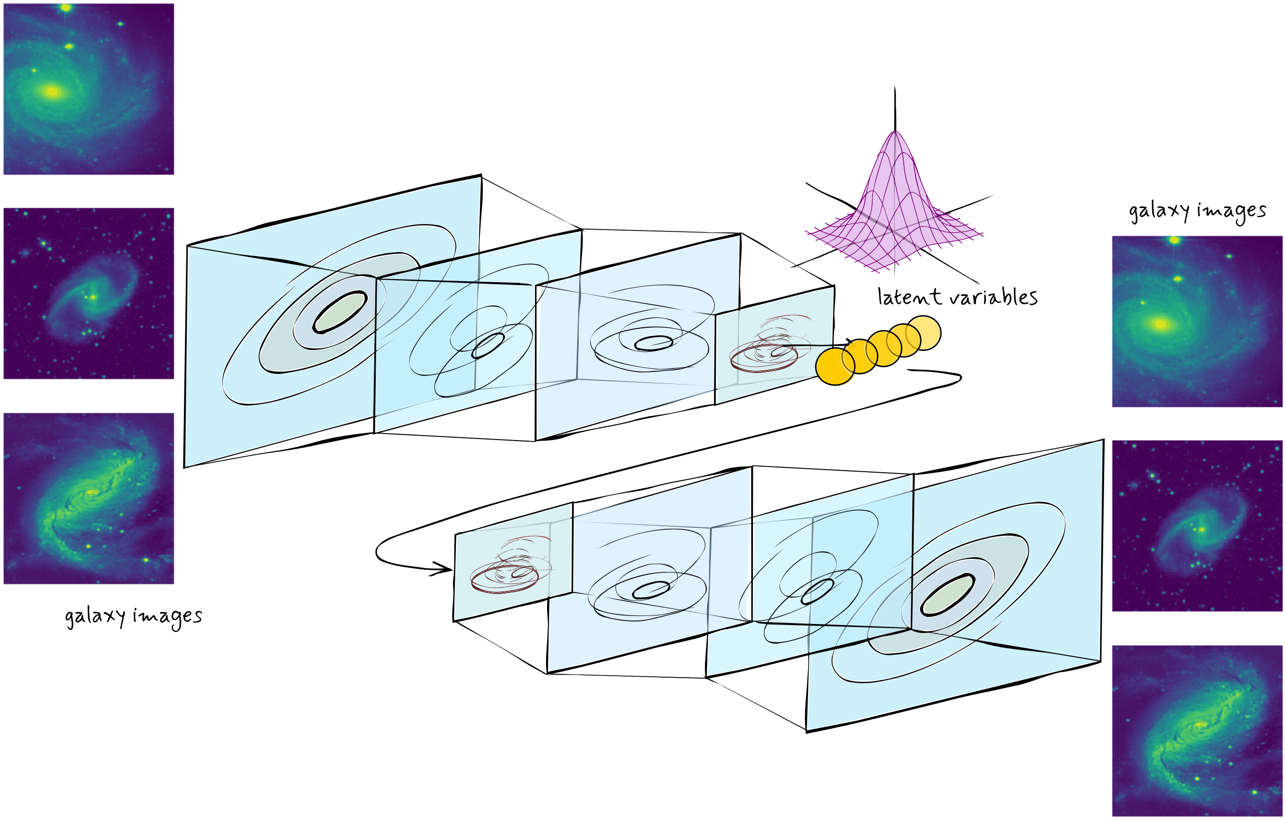
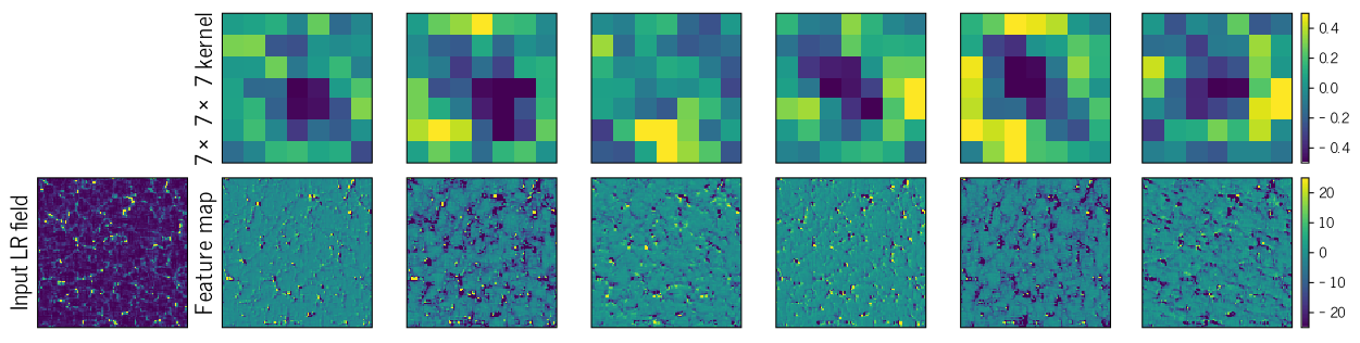
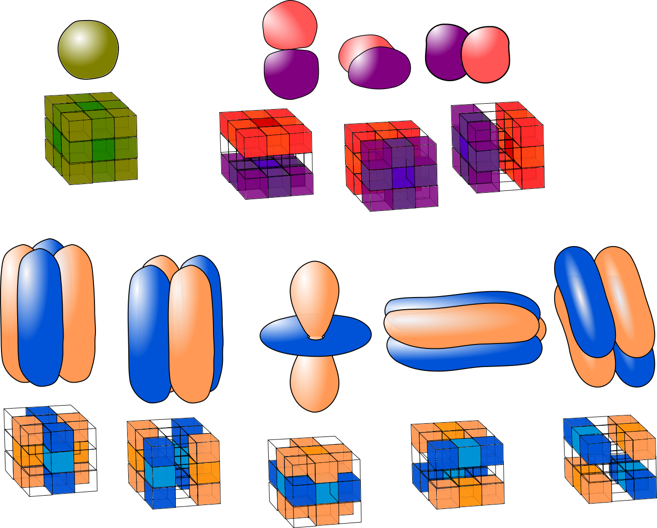
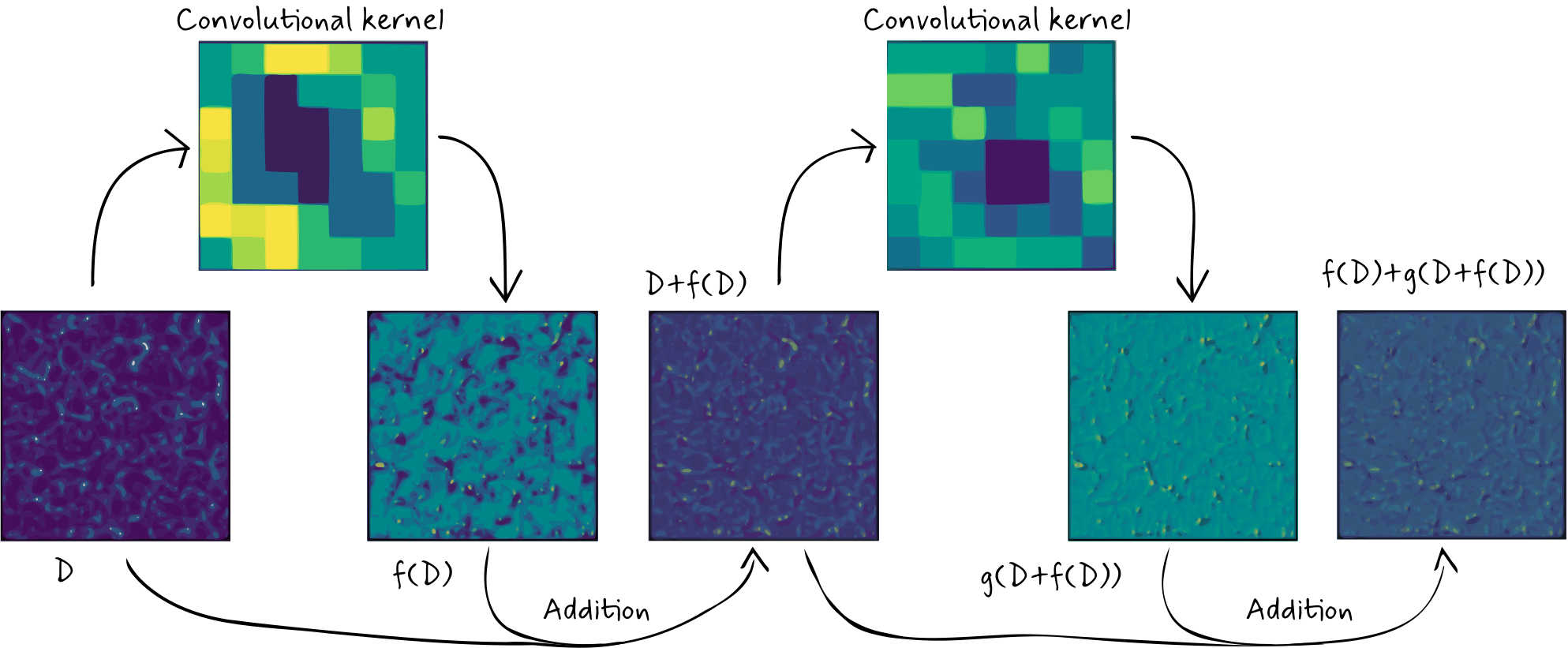
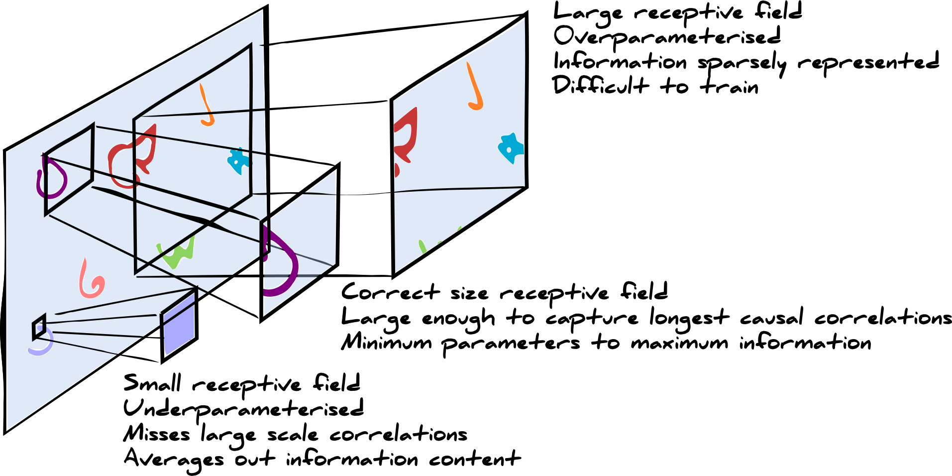
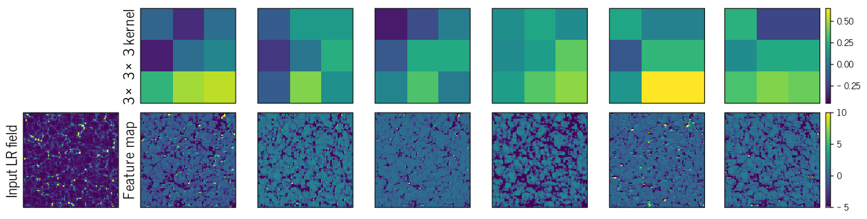
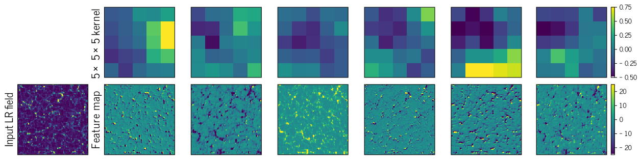
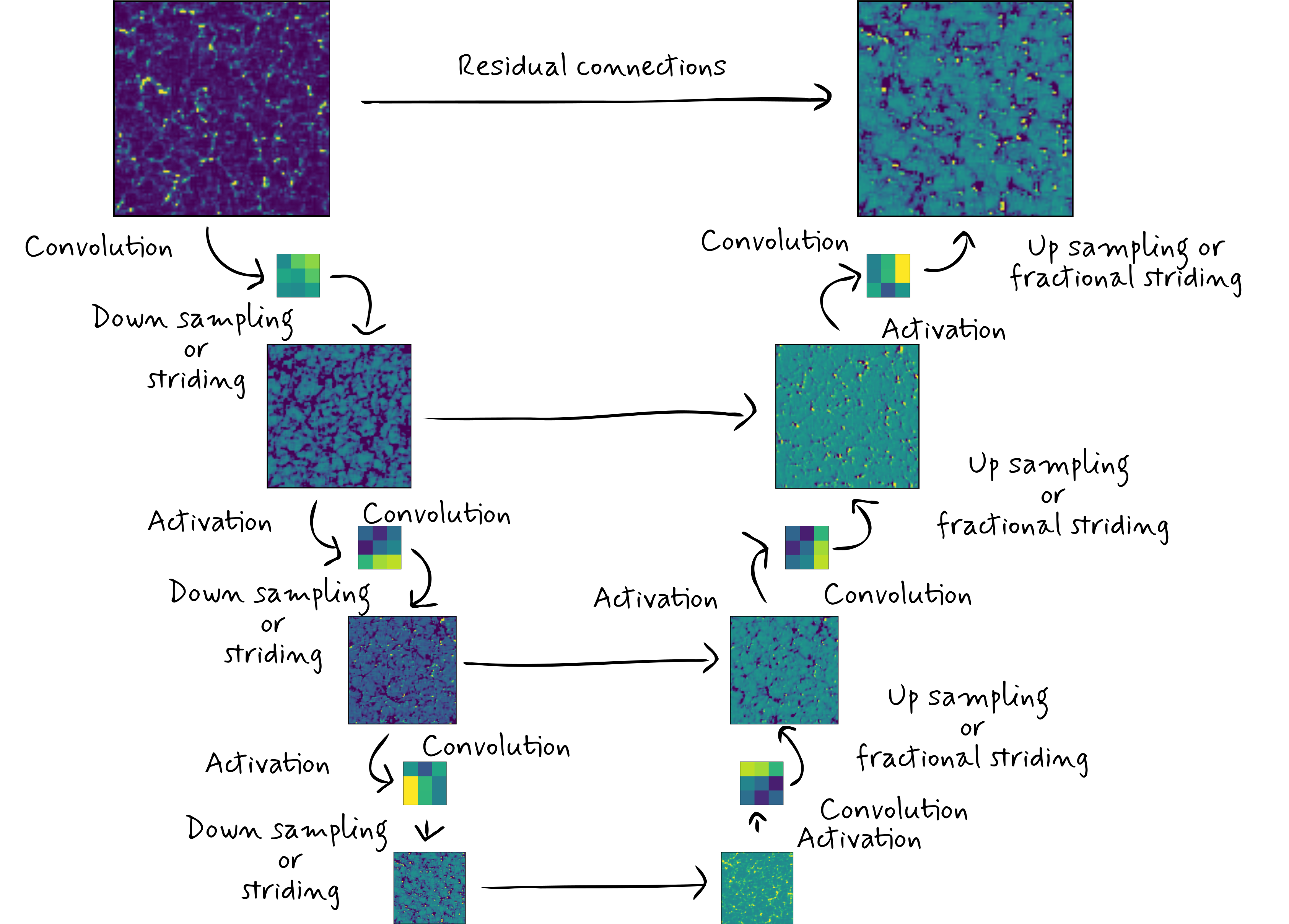
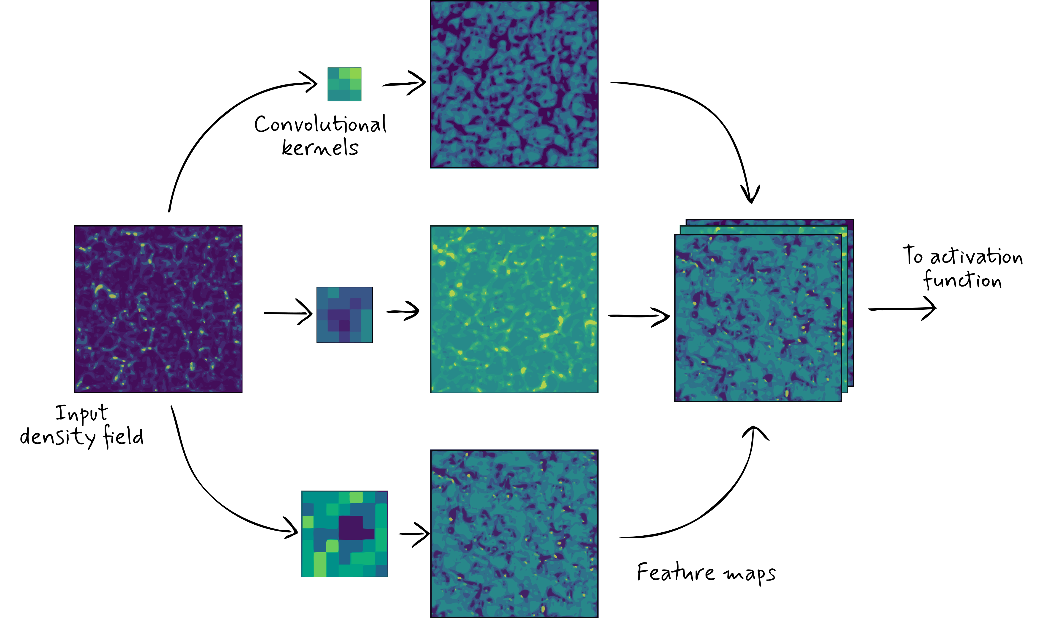
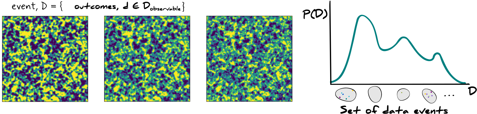
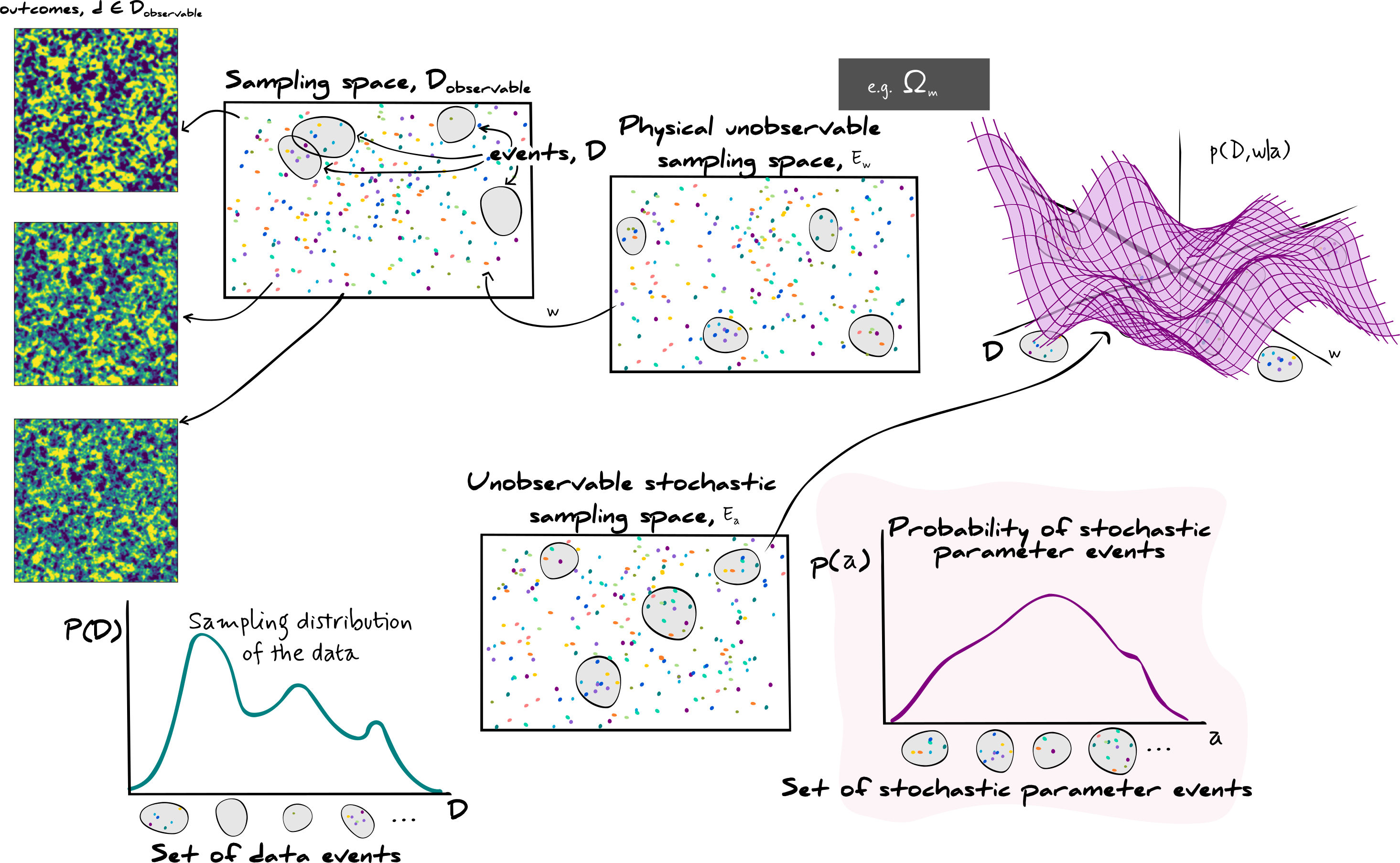
Why do we even care...
we should be talking about neural networks!
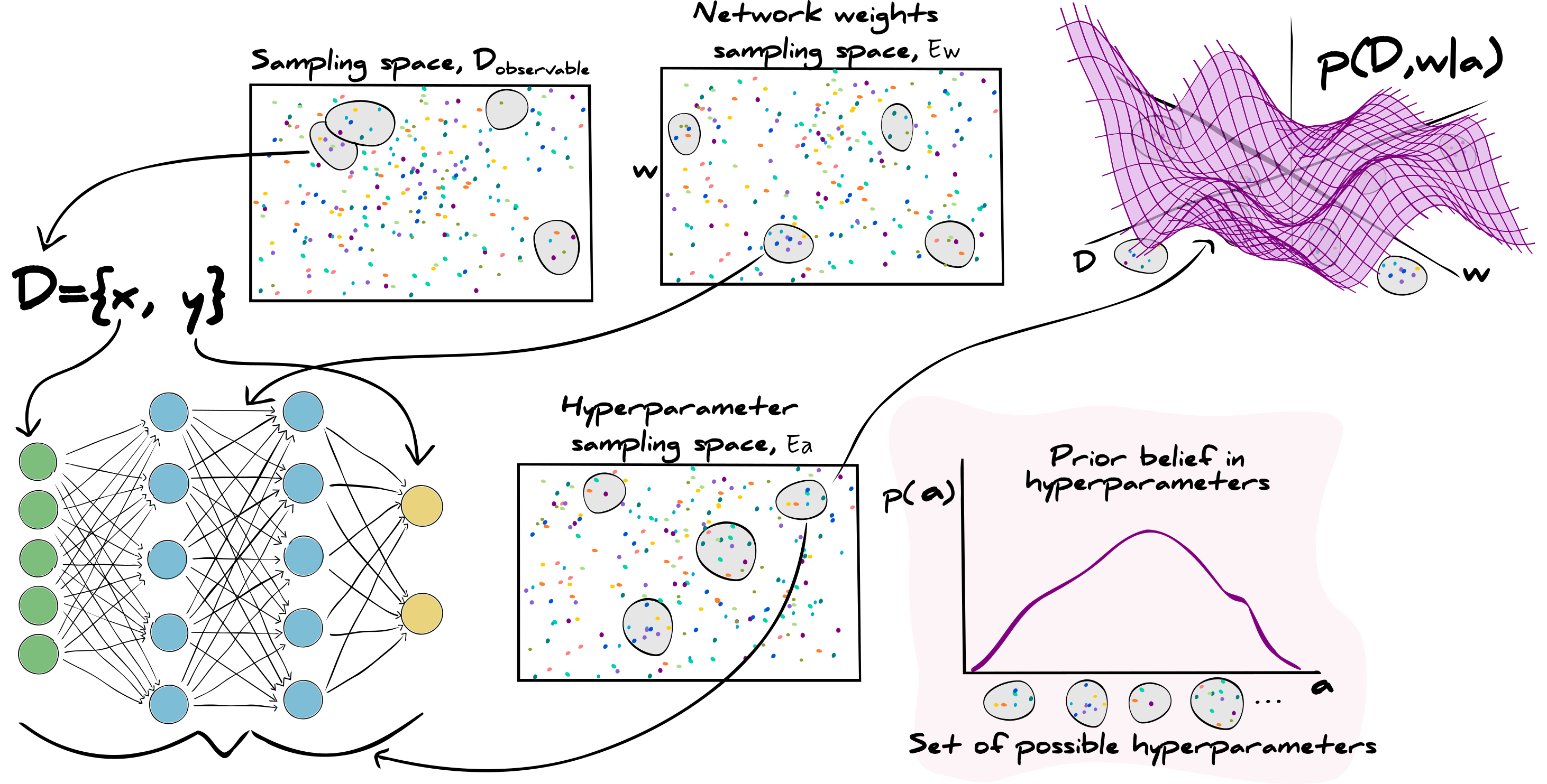
How can we do that?
Variational inference
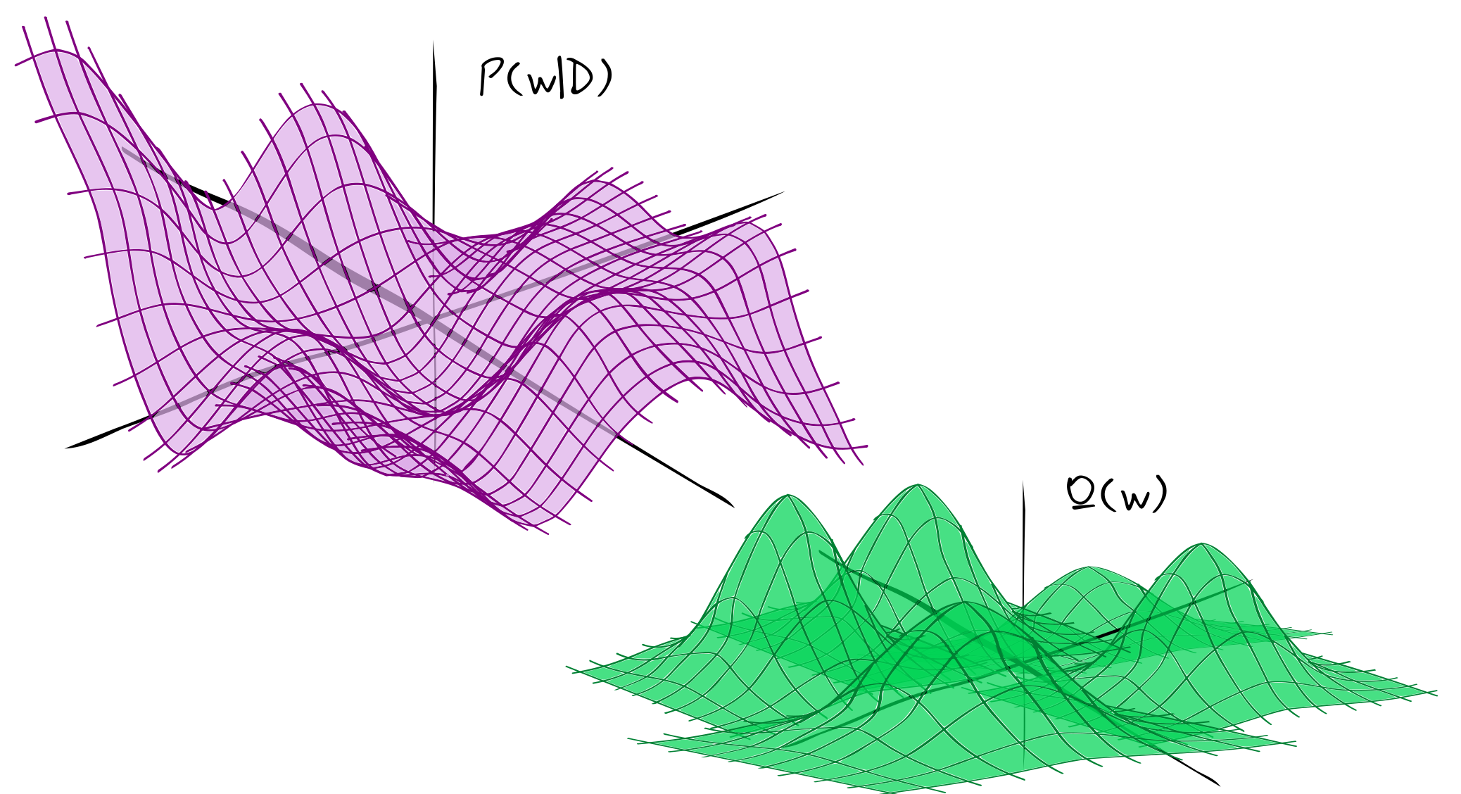
Kullback-Leibler (KL) divergence
A measurement of the information loss by approximating a distribution, $P(y|x)$, with some other distribution, $q(y|x,w,a)$.
$$\mathbb{D}_\textrm{KL}[P(y|x)||q(y|x,w,a)]=\int_{E_y}dyP(y|x)\ln\frac{P(y|x)}{q(y|x,w,a)}$$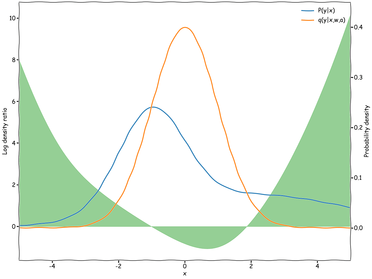
Identical distributions
$$\mathbb{D}_\textrm{KL}[P(y|x)||q(y|x,w,a)]=0\textrm{ means }P(y|x)=q(y|x,w,a)$$Different distributions
$$\mathbb{D}_\textrm{KL}[P(y|x)||q(y|x,w,a)]>0\textrm{ means }P(y|x)\ne q(y|x,w,a)$$Non-symmetric (not a real distance metric)
$$\mathbb{D}_\textrm{KL}[P(y|x)||q(y|x,w,a)]\ne[\mathbb{D}_\textrm{KL}[q(y|x,w,a)||P(y|x)]$$What is the KL-divergence?
$$\begin{align*} \mathbb{D}_\textrm{KL}[P(y|x)||q(y|x,w,a)]&=\int_{E_y}dyP(y|x)\ln\frac{P(y|x)}{q(y|x,w,a)}\\ &=-\int_{E_y}dyP(y|x)\ln q(y|x,w,a)+\int_{E_y}dyP(y|x)\ln P(y|x) \end{align*}$$Entropy of $P(y|x)$
Cross entropy between $P(y|x)$ and $q(y|x,w,a)$
The cross-entropy measures the average number of bits of information needed to tell that an event is drawn from $q(y|x,w,a)$ rather than $P(y|x)$
We don't actually know $P(x,y)$
We might have a sampling distribution, $P(\{x,y\}_\textrm{train})$, made up of
$$\{x_i,y_i\sim P(x,y)|i\in[1,n_\textrm{train}]\}$$(hopefully very close to $\approx P(x,y)$)
Using this sampling distribution we can rewrite the KL divergence as
$$\mathbb{D}_\textrm{KL}[P(y|x)||q(y|x,w,a)]=-\sum_{i=1}^{n_\textrm{train}}P(y_i|x_i)\ln q(y_i|x_i,w,a)+\sum_{i=1}^{n_\textrm{train}}P(y_i|x_i)\ln P(y_i|x_i)$$By minimising the KL-divergence we can attempt to bring $q(y|x,w,a)$ close to $P(y|x)$
(or at least $P(y_\textrm{train}|x_\textrm{train})$).
Entropy term, $P(y|x)$ is independent of $w$, so optimising the parameters of $q(y|x,w,a)$ is equivalent to minimising the cross-entropy
$$\begin{align*} \widehat{w}&=\underset{w\in E_w}{\textrm{arg min}}\,\mathbb{D}_\textrm{KL}[P(y|x)||q(y|x,w,a)]\\ &=\underset{w\in E_w}{\textrm{arg min}}\,-\sum_{i=1}^{n_\textrm{train}}P(y_i|x_i)\ln q(y_i|x_i,w,a) \end{align*}$$How can we calculate the cross entropy?
The likelihood of a training set is
- how often each event, $y_i$, in the training set occurs (or the probability, $P(y_\textrm{train}|x_\textrm{train})$)
- the estimation of the probability using the likelihood, $q(y_i|x_i,w,a)$, for every event
Taking the logarithm (divided by the number of training samples) gives
$$\begin{align*} \frac{1}{n_\textrm{train}}\ln L(y_\textrm{train}|x_\textrm{train})&=\frac{1}{n_\textrm{train}}\ln\prod_{i=1}^{n_\textrm{train}}q(y_i|x_i,w,a)^{n_\textrm{train}P(y_i|x_i)}\\ &=\sum_{i=1}^{n_\textrm{train}}P(y_i|x_i)q(y_i|x_i,w,a) \end{align*}$$Minimising the cross-entropy is equivalent to maximising the logarithm of the likelihood!
Maximum-likelihood estimation!
$$\widehat{w}=\underset{w\in E_w}{\textrm{arg min}}-\ln L(y_\textrm{train}|x_\textrm{train})$$
Equivalent to minimising the KL-divergence and bringing $q(y|x,w,a)$ as close to $P(y|x)$ as possible
False
Neural networks only predict parameters, $Y=f_{w,a}(x)$, of a distribution that we choose.
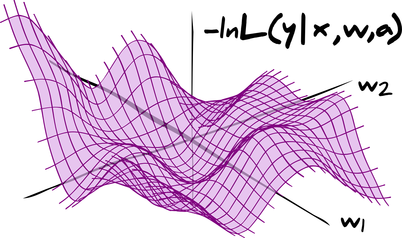
The $Y$ should not be interpreted as predictions of $y$ from $(x, y)$
Example time!
%pylab inline
import jax
import flax
import tqdm
import tensorflow_probability as tfp
import warnings
import os
from scipy.stats import gaussian_kde
warnings.filterwarnings('ignore')
np = jax.numpy
tfp = tfp.experimental.substrates.jax
tfd = tfp.distributions
rng = jax.random.PRNGKey(0)
xkcd();
\\(y = mx + \epsilon\\) where \\(\epsilon\sim\mathbb{N}(0, 1)\\) and \\(x\in[0, 10]\\).
n_train_sims = 1000; x = np.linspace(0, 10, 100).astype(np.float32)

def simulator(m, key):
    return (m * x[np.newaxis, :] + jax.random.normal(key, shape=(m.shape[0],) + x.shape))

rng, key = jax.random.split(rng)
m = jax.random.uniform(key, minval=-5, maxval=5, shape=(n_train_sims, 1))

rng, key = jax.random.split(rng)
y = simulator(m, key)
split = 0.1
m_train = m[:int(n_train_sims * (1 - split))]
y_train = y[:int(n_train_sims * (1 - split))]
m_validate = m[int(n_train_sims * (1 - split)):]
y_validate = y[int(n_train_sims * (1 - split)):]
figure("Training data", figsize=(20, 16)); xlabel("x", fontsize=20); xlim([0, 10]); ylabel("y train", fontsize=20);tick_params(axis="both", labelsize=20)
plot(x, y_train.T[:, ::10], alpha=0.6);

Now lets make a neural network to estimate $m$.
We're going to make two identical networks
- train traditionally
- explicitly characterise a probabilistic model, $L(m|y,w,a)=\mathbb{N}\left(f_{w,a}(y),\mathbb{I}\right)$
@flax.nn.module
def dense_predictor(x):
    x = flax.nn.Dense(x, 128)
    x = flax.nn.leaky_relu(x, 0.01)
    x = flax.nn.Dense(x, 128)
    x = flax.nn.leaky_relu(x, 0.01)
    x = flax.nn.Dense(x, 1)
    return x

rng, key = jax.random.split(rng)
_, initial_params = dense_predictor.init_by_shape(
    key, [((100,), np.float64)])

mse_model = flax.nn.Model(dense_predictor, initial_params)
mse_opt = flax.optim.Adam(1e-5).create(mse_model)

tfp_model = flax.nn.Model(dense_predictor, initial_params)
tfp_opt = flax.optim.Adam(7e-6).create(tfp_model)
So classically we might want to regress to the esimate using mean squared error as a loss function $$\Lambda = \frac{1}{N}\sum_{i=1}^N(f_{w,a}(y_i)-m_i)^2$$
@jax.jit
def mse(y, m, model):
    def fn(y, m):
        return np.mean((model(y) - m)**2.)
    return np.mean(jax.vmap(fn)(y, m))
Lets also maximise the log likelihood, i.e. minimise the cross entropy, i.e.i.e minimise the KL divergence
@jax.jit
def negloglike(y, m, model):
    def fn(y, m):
        return np.mean(-tfd.Normal(loc=model(y), scale=1).log_prob(m))
    return np.mean(jax.vmap(fn)(y, m))
Now we do the optimisation of the weights via backpropagation
$$\begin{align*} w_i&\leftarrow w_i+\eta\partial_{w_i}\textrm{MSE}(f_{w,a}(y_\textrm{train}), m_\textrm{train})\\ w_i&\leftarrow w_i+\eta\partial_{w_i}-\ln\mathbb{N}(f_{w,a}(y_\textrm{train}), \mathbb{I}|m_\textrm{train}) \end{align*}$$(Actually we're going to use Adam, but you get the idea)
@jax.jit
def optimise(mse_opt, tfp_opt):
    def get_mse(model):
        return mse(y_train, m_train, model)
    def get_negloglike(model):
        return negloglike(y_train, m_train, model)
    mse_loss, mse_grad = jax.value_and_grad(get_mse)(mse_opt.target)
    negloglike_loss, negloglike_grad = jax.value_and_grad(get_negloglike)(tfp_opt.target)
    mse_opt = mse_opt.apply_gradient(mse_grad)
    tfp_opt = tfp_opt.apply_gradient(negloglike_grad)
    return mse_opt, tfp_opt, [mse_loss, negloglike_loss]
And fit the models (for 1000 epochs) (we'll also validate the network with our unseen validation set to evaluate the performance)
epochs = 1000; loss = []; val_loss = []; bar = tqdm.tnrange(epochs, desc="iterations")
for i in bar:
    mse_opt, tfp_opt, loss_ = optimise(mse_opt, tfp_opt)
    loss.append(loss_)
    val_loss.append([
        mse(y_validate, m_validate, mse_opt.target),
        negloglike(y_validate, m_validate, tfp_opt.target)])
    bar.set_postfix(loss=loss[i], val_loss=val_loss[i])
loss = np.array(loss); val_loss = np.array(val_loss)
n_test_sims = 100

rng, key = jax.random.split(rng)
m_test = jax.random.uniform(key, minval=-5, maxval=5, shape=(n_test_sims, 1))

rng, key = jax.random.split(rng)
y_test = simulator(m_test, key)

m_predicted = mse_opt.target(y_test)
m_estimated_mean = tfd.Normal(tfp_opt.target(y_test), scale=1).mean()
figure("Predicted m", figsize=(20, 16)); plot([-5, 5], [-5, 5], linestyle="dashed", color="black",linewidth=3); xlabel("m predicted", fontsize=20); xlim([-5, 5]); ylabel("m test", fontsize=20); ylim([-5, 5]); tick_params(axis="both", labelsize=20)
scatter(m_predicted, m_test, color="C0", s=250, label="MSE")
scatter(m_estimated_mean, m_test, color="C1", marker="+", s=250, label="log P(m|y)")
legend(fontsize=20);

So network outputs are just the parameters of a probabilistic model that we choose as a description of our problem
Using the MSE is equivalent to saying that you believe the distribution, $P(y|x)$, is able to be modelled as a Gaussian with locations given by the network output.
(whether or not this is a good choice is a different question)
Note that the same is true for minimising the binary cross-entropy
- Equivalent to fitting the parameters of a Bernoulli distribution to minimise the KL divergence, $P(y|x)\approx q(y|x,w,a)=\textrm{Bernoulli}(f_{w,a}(x))$
And minimising absolute error
- Equivalent to fitting the parameters of a Laplacian distribution to minimise the KL diverenge, $P(y|x)\approx q(y|x,w,a)=\textrm{Laplacian}(f_{w,a}(x))$
Training a neural network is doing variational inference
Since we have made a stochastic model, $q(y|x,\widehat{w},a)$, of $P(y|x)$ we get estimated uncertainties of $y$ for free
figure("Probabilistic model for m", figsize=(20, 16)); plot([-5, 5], [-5, 5], color="black", linestyle="dashed", linewidth=3); xlim([-4, 4]); xlabel("m predicted", fontsize=20); ylim([-4, 4]); ylabel("m test", fontsize=20); tick_params(axis="both", labelsize=20); m_eval = np.linspace(-5, 5, 100).reshape(1, 1, -1);
contourf(m_eval[0, 0], m_test[:, 0], tfd.Normal(tfp_opt.target(y_test), scale=1).prob(m_eval)[0], levels=50)
cbar = colorbar(); cbar.set_label("P(m|y)", fontsize=20); cbar.ax.tick_params(labelsize=20)
scatter(tfd.Normal(tfp_opt.target(y_test), scale=1).mean(), m_test[:, 0], s=100);

Note this doesn't tell us if our estimate is actually any good.
- Specifically, because we only calculate the cross entropy, we ignore the entropy in the minimisation of the KL-divergence, whose calculation would actually tell us whether the distributions were identical.
- Note that this is only true for the sampling distribution of data that we have and not the true distribution of all possible data.
When comparing different models we tend to use statistics such as the Bayesian evidence ratio
$\displaystyle B = (\ln)\frac{p(D|a_2)}{p(D|a_1)}$
As physicists we prefer some quantification of simplicity (Occam's razor)
- $BIC = k\ln n - 2\ln L(D|w^*, a)$
- $AIC = 2k - 2\ln L(D|w^*, a)$
i.e. we prefer ΛCDM over a polynomial fit with tons of parameters and fits the data perfectly, but is not predictive.
Neural networks will always lose at model comparison stage
Although predictions can be validated using a test set there is no physical principle which will tell us the general behaviour for any new piece of data... we just have to hope!
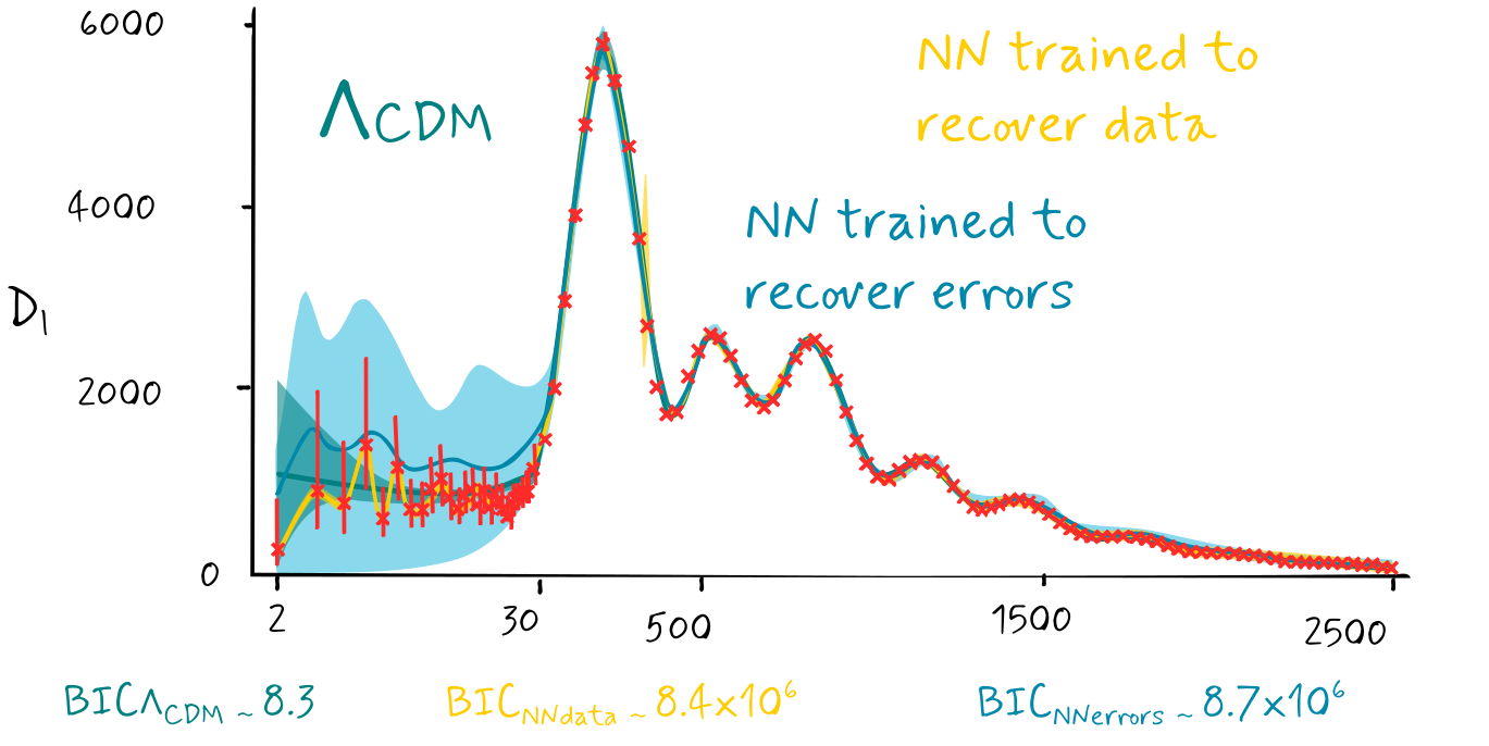
Using any sensible criterion for model selection a neural network with it's loss function will always be rejected on parameter counts and the lack of predictability.
Is there any hope for using machine learning?
Of course there is...
We can see that neural networks are able to extract ridiculously large amounts of information directly from the data.
We just need to use the extracted information in a way that does not depend on the neural network as a model, just as a function.
Likelihood-free inference (ask me later)
Machine learning to accelerate science (example, FLEET 2020)
There are many times that we can use machine learning to accelerate the way that we obtain data which we can use for science, rather than using the network itself for science.
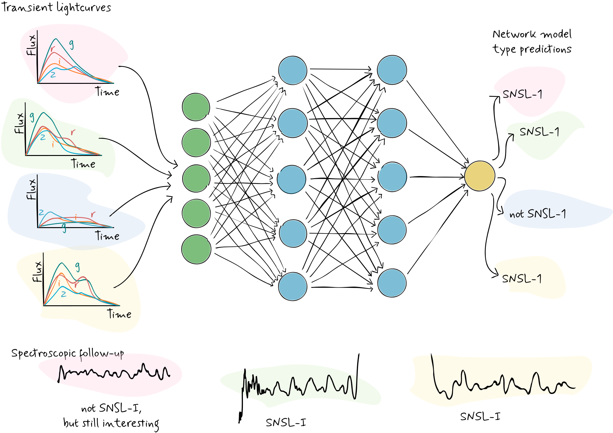
Neural networks using in a Bayesian setting
(Charnock, Lavaux, Wandelt, Sarma Boruah, Jasche and Hudson 2020)
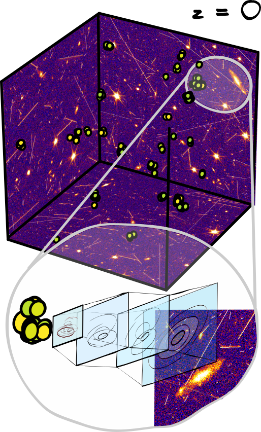
- Forward model all understood physics
- Make abstract function (NN) made from physically motivated architecture choice
- Remove all unidentifiable weights
- Use high dimensional Markov methods to sample physical properties AND neural network weights
Not deep learning anymore - we're just benefitting from the differentiable frameworks and doing old-school* physics 😉

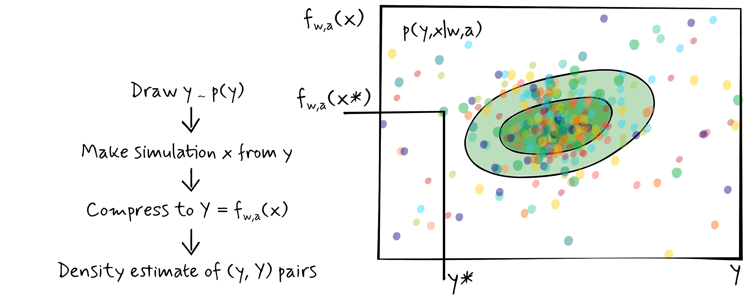
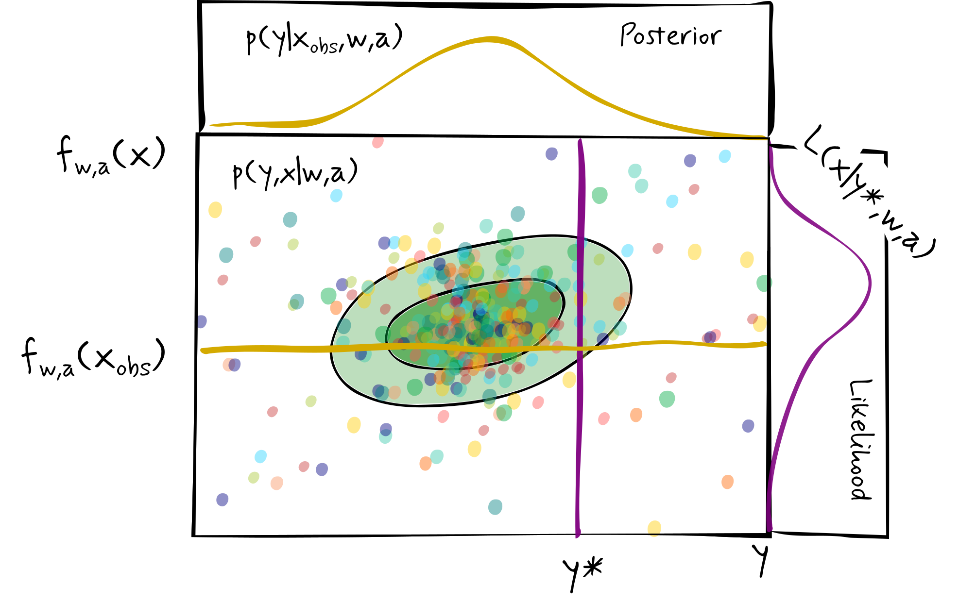
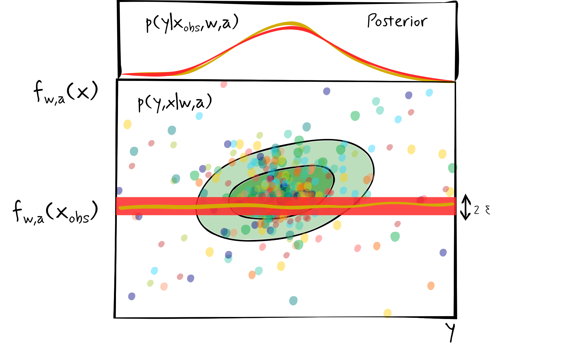
Approximate Bayesian computation (ABC)
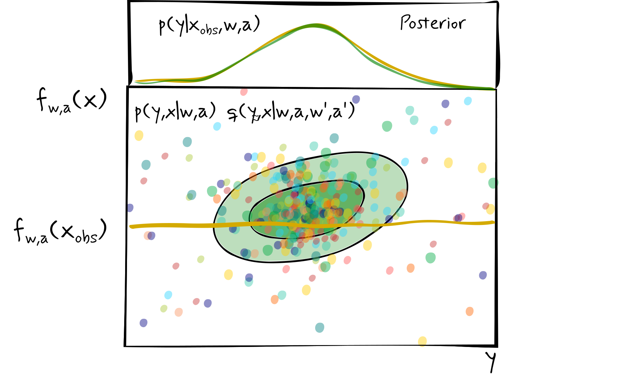
Density estimate likelihood-free inference (DELFI)
Another example - yay!
n_LFI = int(1e5)

rng, key = jax.random.split(rng)
m_LFI = jax.random.uniform(key, minval=-5, maxval=5, shape=(n_LFI, 1))
rng, key = jax.random.split(rng)
t_LFI = mse_opt.target(simulator(m_LFI, key))
DELFI_LFI = gaussian_kde(np.concatenate([m_LFI, t_LFI], axis=-1).T)

m_obs = m_test[3, 0]
t_obs = mse_opt.target(y_test[3])[0]
ϵ_LFI = 0.1
bins = 100
fig, ax = subplots(2, 2, figsize=(20, 20)); ax[0, 1].axis("off"); ax[1, 0].set_xlabel("m", fontsize=20), ax[1, 0].set_ylabel("t", fontsize=20);ax[1, 1].set_xlabel("L(t|m obs, w, a)", fontsize=20);ax[0, 0].set_ylabel("P(m|y obs, w, a)", fontsize=20);subplots_adjust(wspace=0, hspace=0);ax[0, 0].set_xticks([]);ax[1, 1].set_yticks([]);ax[0, 0].set_xlim([-5, 5]);ax[1, 0].set_xlim([-5, 5]);ax[1, 0].set_ylim([-5, 5]);ax[1, 1].set_ylim([-5, 5]);ax[0, 0].tick_params(axis="both", labelsize=20);ax[1, 0].tick_params(axis="both", labelsize=20);ax[1, 1].tick_params(axis="both", labelsize=20)
ax[0, 0].axvline(m_test[3], linestyle="dashed", color="C0", linewidth=3, label="m obs");ax[0, 0].plot(np.linspace(-5, 5, 1000), DELFI_LFI(np.vstack([np.linspace(-5, 5, 1000), np.repeat(t_obs, 1000)]))/0.1, color="C2", linestyle="dotted", label="NN DELFI posterior");ax[0, 0].hist(m_LFI.T[(t_LFI.T>t_obs-ϵ_LFI)*(t_LFI.T<t_obs+ϵ_LFI)], range=[m_LFI.min(), m_LFI.max()], bins=bins, density=True, histtype='step', linewidth=3, color="C2", label="NN ABC posterior");ax[0, 0].legend(fontsize=20)
ax[1, 1].axhline(t_obs, linestyle="dashed", color="C2", linewidth=3);ax[1, 1].hist(t_LFI.T[(m_LFI.T>m_obs-ϵ_LFI)*(m_LFI.T<m_obs+ϵ_LFI)], range=[t_LFI.min(), t_LFI.max()], bins=bins, density=True, histtype='step', orientation="horizontal", linewidth=3, color="C2",label="NN ABC likelihood");ax[1, 1].plot(DELFI_LFI(np.vstack([np.repeat(m_obs, 1000), np.linspace(-5, 5, 1000)]))/0.1, np.linspace(-5, 5, 1000), color="C2", linestyle="dotted", label="NN DELFI likelihood");ax[1, 1].legend(fontsize=20)
ax[1, 0].scatter(m_LFI, t_LFI,s=1, alpha=0.5,c="C2");ax[1, 0].fill_between([-5, 5], [t_obs-ϵ_LFI, t_obs-ϵ_LFI], [t_obs+ϵ_LFI, t_obs+ϵ_LFI], color="C2",edgecolor=None,alpha=0.5);ax[1, 0].fill_between([t_obs-ϵ_LFI, t_obs+ϵ_LFI], [-5, -5], [5, 5], color="C2",edgecolor=None,alpha=0.5);ax[1, 0].axvline(m_test[3], linestyle="dashed", color="C0", linewidth=3);

Information maximising neural networks
(Charnock, Lavaux and Wandelt 2018)
Completely different use for network (not modelling)
Find the function which maximises the information about your parameters
- Don't actually care what the network outputs, but we can make them nice, i.e. Gaussianly distributed, etc.
This makes use of the deep learning framework, and the neural network, but for a very different purpose!
Gaussian Fisher information
$$\begin{align*} {\bf F}_{\alpha\beta} &= \left.\left\langle\frac{\partial\ln L(x|y)}{\partial y_\alpha}\frac{\partial\ln L(x|y)}{\partial y_\beta}\right\rangle\right|_{y=y^\textrm{fid}}\\ &=\frac{\partial\mu(y)}{\partial y_\alpha}^T{\bf C}^{-1}\frac{\partial\mu(y)}{\partial y_\beta} \end{align*}$$If we do not know the likelihood $L(x|y)$, transform the data using a neural network to get the likelihood $L(z|y,w,a)$ , where $z=f_{w,a}(x)$
Then maximise $\ln\det{\bf F}_{\alpha\beta}$ where
$${\bf F}_{\alpha\beta} = \frac{\partial\mu(f_{w,a}(x(y)))}{\partial y_\alpha}^T{\bf C}(f_{w,a}(x(y)))^{-1}\frac{\partial\mu(f_{w,a}(x(y)))}{\partial y_\beta}$$Calculate the mean of the derivative of the network outputs with respect to the parameters, $\displaystyle \frac{\partial\mu(f_{w,a}(x(y)))}{\partial y_\alpha}$
Calculate the covariance of the network outputs with respect to the parameters, ${\bf C}(f_{w,a}(x(y)))$
We also want to set the scale of the summaries which we can do with a regulariser (which is arbitrary) like $$\Lambda_2 = \|{\bf C}(f_{w,a}(x(y)))-\mathbb{I}\|+\|{\bf C}(f_{w,a}(x(y)))-\mathbb{I}\|$$
This is all very easy to do using modern frameworks
A last example
rng, key = jax.random.split(rng)
_, initial_params = dense_predictor.init_by_shape(
    key, [((100,), np.float64)])
IMNN_model = flax.nn.Model(dense_predictor, initial_params)
IMNN_opt = flax.optim.Adam(1e-3).create(IMNN_model)
n_s = 1000; n_d=n_s; λ = 10; ϵ = 0.01; α = -np.log((λ - 1) * ϵ + ϵ**2. / (1 + ϵ)) / ϵ
rng, key = jax.random.split(rng)
m_IMNN = np.array([[0]])
δm_IMNN = 0.1
y_IMNN = simulator(np.repeat(m_IMNN, n_s, axis=0), key)
y_d_IMNN = np.concatenate(
    [simulator(np.repeat(m_IMNN-δm_IMNN/2, n_d, axis=0), key)[:, np.newaxis, np.newaxis, :],
     simulator(np.repeat(m_IMNN+δm_IMNN/2, n_d, axis=0), key)[:, np.newaxis, np.newaxis, :]],
    axis=1)
rng, key = jax.random.split(rng)
val_y_IMNN = simulator(np.repeat(m_IMNN, n_s, axis=0), key)
val_y_d_IMNN = np.concatenate(
    [simulator(np.repeat(m_IMNN-δm_IMNN/2, n_d, axis=0), key)[:, np.newaxis, np.newaxis, :],
     simulator(np.repeat(m_IMNN+δm_IMNN/2, n_d, axis=0), key)[:, np.newaxis, np.newaxis, :]],
    axis=1)
@jax.jit
def regulariser(C, invC):
    Λ2 = np.sum((C-np.eye(1))**2.) + np.sum((invC-np.eye(1))**2.)
    r = λ * Λ2 / (Λ2 + np.exp(-α * Λ2))
    return Λ2, r

@jax.jit
def Fisher(model, y, y_d):
    t = model(y)
    t_d = model(y_d)
    dμ_dm = np.mean((t_d[:, 1] - t_d[:, 0]) / δm_IMNN, 0)
    μ = np.mean(t, axis=0)
    C = np.cov(t, rowvar=False)[np.newaxis, np.newaxis]
    invC = np.linalg.inv(C)
    F = np.einsum("ij,jk,lk->il", dμ_dm, invC, dμ_dm)
    return F, C, invC, μ, dμ_dm

@jax.jit
def IMNN_loss(model):
    F, C, invC, _, _ = Fisher(model, y_IMNN, y_d_IMNN)
    lndetF = np.linalg.slogdet(F)
    Λ2, r = regulariser(C, invC)
    return - lndetF[0] * lndetF[1] + r * Λ2

@jax.jit
def IMNN_optimise(IMNN_opt):
    F_grad = jax.grad(IMNN_loss)(IMNN_opt.target)
    IMNN_opt = IMNN_opt.apply_gradient(F_grad)
    return IMNN_opt
if os.path.isfile("data/IMNN_opt.npy"):
    epochs = 5
    IMNN_opt = flax.serialization.from_state_dict(IMNN_opt, np.load("data/IMNN_opt.npy", allow_pickle=True)[()])
    detF_ = [i for i in np.load("data/detF.npy")]
    val_detF_ = [i for i in np.load("data/val_detF.npy")]
    detC_ = [i for i in np.load("data/detC.npy")]
    val_detC_ = [i for i in np.load("data/val_detC.npy")]
    detinvC_ = [i for i in np.load("data/detinvC.npy")]
    val_detinvC_ = [i for i in np.load("data/val_detinvC.npy")]
    r_ = [i for i in np.load("data/r.npy")]
    val_r_ = [i for i in np.load("data/val_r.npy")]
else:
    epochs = 400
    detF_ = [];
    val_detF_ = [];
    detC_ = [];
    val_detC_ = [];
    detinvC_ = [];
    val_detinvC_ = [];
    r_ = [];
    val_r_ = [];
bar = tqdm.tnrange(epochs, desc="iterations")
for i in bar:
    IMNN_opt = IMNN_optimise(IMNN_opt)
    F_temp, C_temp, invC_temp, _, _ = Fisher(IMNN_opt.target, y_IMNN, y_d_IMNN)
    Λ2_temp, r_temp = regulariser(C_temp, invC_temp)
    detF_.append(np.linalg.det(F_temp))
    detC_.append(np.linalg.det(C_temp))
    detinvC_.append(np.linalg.det(invC_temp))
    r_.append(r_temp)
    F_temp, C_temp, invC_temp, _, _ = Fisher(IMNN_opt.target, val_y_IMNN, val_y_d_IMNN)
    Λ2_temp, r_temp = regulariser(C_temp, invC_temp)
    val_detF_.append(np.linalg.det(F_temp))
    val_detC_.append(np.linalg.det(C_temp))
    val_detinvC_.append(np.linalg.det(invC_temp))
    val_r_.append(r_temp)
    bar.set_postfix(detF=detF_[-1], val_detF=val_detF_[-1], detC=detC_[-1], val_detC=val_detC_[-1], r=r_[-1], val_r=val_r_[-1])
#np.save("data/detF.npy", detF_);np.save("data/val_detF.npy", val_detF_);np.save("data/detC.npy", detC_);np.save("data/val_detC.npy", val_detC_);np.save("data/detinvC.npy", detinvC_);np.save("data/val_detinvC.npy", val_detinvC_);np.save("data/r.npy", r_);np.save("data/val_r.npy", val_r_);np.save("data/IMNN_opt.npy", flax.serialization.to_state_dict(IMNN_opt))
fig, ax = subplots(1, 3, figsize=(32,10));ax_ = ax[1].twinx();ax[0].set_xlabel("Epochs", fontsize=20);ax[0].set_ylabel("$|F|$", fontsize=20);ax[1].set_xlabel("Epochs", fontsize=20);ax[1].set_ylabel("$|C|$", fontsize=20);ax_.set_ylabel("$|C^{-1}|$", fontsize=20);ax[2].set_xlabel("Epochs", fontsize=20);ax[2].set_ylabel("$r$", fontsize=20);ax[0].tick_params(axis="both", labelsize=20);ax[1].tick_params(axis="both", labelsize=20);ax_.tick_params(axis="both", labelsize=20);ax[2].tick_params(axis="both", labelsize=20);epo2 = np.arange(1, len(detF_)+1);ax[0].set_xlim([1, len(detF_)]);ax[1].set_xlim([1, len(detF_)]);ax[2].set_xlim([1, len(detF_)]);subplots_adjust(wspace=0.5)
ax[0].plot(epo2, detF_, linewidth=3)
ax[0].plot(epo2, val_detF_, linewidth=3)
ax[1].plot(epo2, detC_, linewidth=3)
ax[1].plot(epo2, val_detC_, linewidth=3)
ax_.plot(epo2, detinvC_, linestyle="dashed", linewidth=3)
ax_.plot(epo2, val_detinvC_, linestyle="dashed", linewidth=3)
ax[2].plot(epo2, r_, linewidth=3)
ax[2].plot(epo2, val_r_, linewidth=3);

F, C, invC, μ, dμ_dm = Fisher(IMNN_opt.target, val_y_IMNN, val_y_d_IMNN)
invF = np.linalg.inv(F)

@jax.jit
def IMNN_estimator(y):
    return m_IMNN + np.einsum("ij,jk,kl,ml->mi", invF, dμ_dm, invC, (IMNN_opt.target(y) - μ))

rng, key = jax.random.split(rng)
t_IMNN = IMNN_estimator(simulator(m_LFI, key))
DELFI_IMNN = gaussian_kde(np.concatenate([m_LFI, t_IMNN], axis=-1).T)

t_IMNN_obs = IMNN_estimator(y_test[3:4])[0, 0]

ϵ_IMNN = 0.01
fig, ax = subplots(2, 2, figsize=(20, 20)); ax[0, 1].axis("off"); ax[1, 0].set_xlabel("m", fontsize=20), ax[1, 0].set_ylabel("t", fontsize=20);ax[1, 1].set_xlabel("$\mathcal{L}(t|m_{obs}, \widehat{w},\widehat{a})$", fontsize=20);ax[0, 0].set_ylabel("$\mathcal{P}(m|y_{obs}, \widehat{w},\widehat{a})$", fontsize=20);subplots_adjust(wspace=0, hspace=0);ax[0, 0].set_xticks([]);ax[1, 1].set_yticks([]);ax[0, 0].set_xlim([-5, 5]);ax[1, 0].set_xlim([-5, 5]);ax[1, 0].set_ylim([-5, 5]);ax[1, 1].set_ylim([-5, 5]);ax[0, 0].tick_params(axis="both", labelsize=20);ax[1, 0].tick_params(axis="both", labelsize=20);ax[1, 1].tick_params(axis="both", labelsize=20)
ax[0, 0].axvline(m_test[3], linestyle="dashed", color="C0", linewidth=3, label="m obs");ax[0, 0].hist(m_LFI.T[(t_LFI.T>t_obs-ϵ_LFI)*(t_LFI.T<t_obs+ϵ_LFI)], range=[m_LFI.min(), m_LFI.max()], bins=bins, density=True, histtype='step', linewidth=3, color="C2",label="NN ABC posterior");ax[0, 0].plot(np.linspace(-5, 5, 1000), DELFI_LFI(np.vstack([np.linspace(-5, 5, 1000), np.repeat(t_obs, 1000)]))/0.1, linestyle="dotted", color="C2", label="NN DELFI posterior");ax[0, 0].hist(m_LFI.T[(t_IMNN.T>t_IMNN_obs-ϵ_IMNN)*(t_IMNN.T<t_IMNN_obs+ϵ_IMNN)], range=[m_LFI.min(), m_LFI.max()], bins=bins, density=True, histtype='step', linewidth=3, color="C1",label="IMNN ABC posterior");ax[0, 0].plot(np.linspace(-5, 5, 1000), DELFI_IMNN(np.vstack([np.linspace(-5, 5, 1000), np.repeat(t_obs, 1000)]))/0.1, color="C1", linestyle="dotted", label="IMNN DELFI posterior");ax[0, 0].legend(fontsize=20)
ax[1, 1].axhline(t_obs, linestyle="dashed", color="C2", linewidth=3, alpha=0.5);ax[1, 1].axhline(t_IMNN_obs, linestyle="dashed", color="C1", linewidth=3, alpha=0.5);ax[1, 1].hist(t_LFI.T[(m_LFI.T>m_obs-ϵ)*(m_LFI.T<m_obs+ϵ)], range=[t_LFI.min(), t_LFI.max()], bins=bins, density=True, histtype='step', orientation="horizontal", linewidth=3, color="C2",label="NN ABC likelihood");ax[1, 1].plot(DELFI_LFI(np.vstack([np.repeat(m_obs, 1000), np.linspace(-5, 5, 1000)]))/0.1, np.linspace(-5, 5, 1000), linestyle="dotted", color="C2", label="NN DELFI likelihood");ax[1, 1].hist(t_IMNN.T[(t_IMNN.T>t_IMNN_obs-ϵ_IMNN)*(t_IMNN.T<t_IMNN_obs+ϵ_IMNN)], range=[t_IMNN.min(), t_IMNN.max()], bins=bins, density=True, histtype='step', orientation="horizontal", linewidth=3, color="C1",label="IMNN ABC likelihood");ax[1, 1].plot(DELFI_IMNN(np.vstack([np.repeat(m_obs, 1000), np.linspace(-5, 5, 1000)]))/0.1, np.linspace(-5, 5, 1000), color="C1", linestyle="dotted", label="IMNN DELFI likelihood");ax[1, 1].legend(fontsize=20)
ax[1, 0].scatter(m_LFI, t_LFI,s=1, alpha=0.5,c="C2");ax[1, 0].fill_between([-5, 5], [t_obs-ϵ_LFI, t_obs-ϵ_LFI], [t_obs+ϵ_LFI, t_obs+ϵ_LFI], color="C2",edgecolor=None,alpha=0.5);ax[1, 0].fill_between([t_obs-ϵ_LFI, t_obs+ϵ_LFI], [-5, -5], [5, 5], color="C2",edgecolor=None,alpha=0.5);ax[1, 0].scatter(m_LFI, t_IMNN, s=1, alpha=0.5,c="C1");ax[1, 0].fill_between([-5, 5], [t_IMNN_obs-ϵ_IMNN, t_IMNN_obs-ϵ_IMNN], [t_IMNN_obs+ϵ_IMNN, t_IMNN_obs+ϵ_IMNN], color="C1",edgecolor=None,alpha=0.5);ax[1, 0].fill_between([t_IMNN_obs-ϵ_IMNN, t_IMNN_obs+ϵ_IMNN], [-5, -5], [5, 5], color="C1",edgecolor=None,alpha=0.5);ax[1, 0].axvline(m_test[3], linestyle="dashed", color="C0", linewidth=3);

Scientific examples
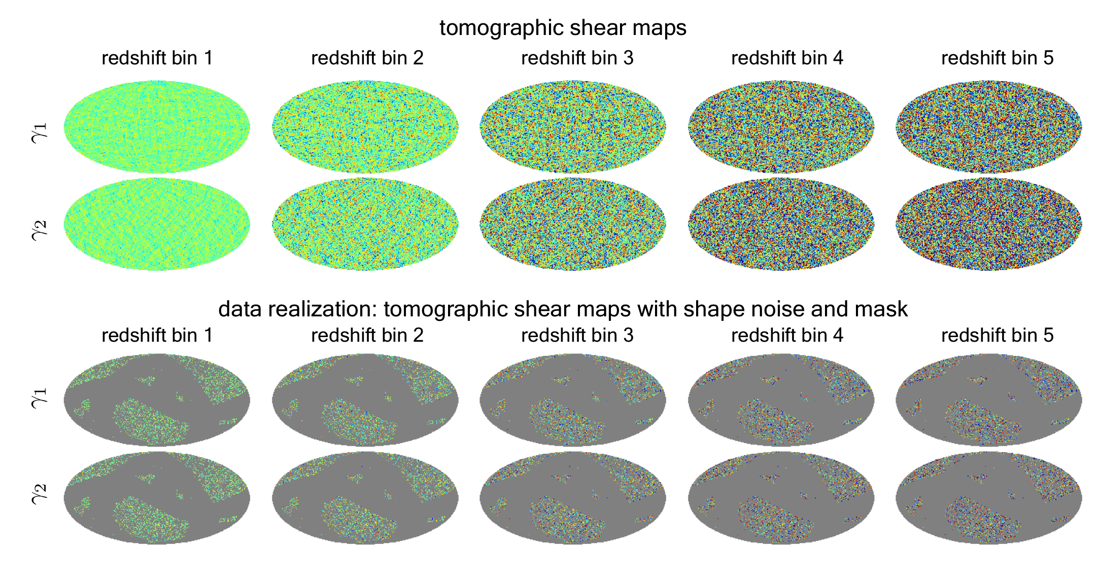
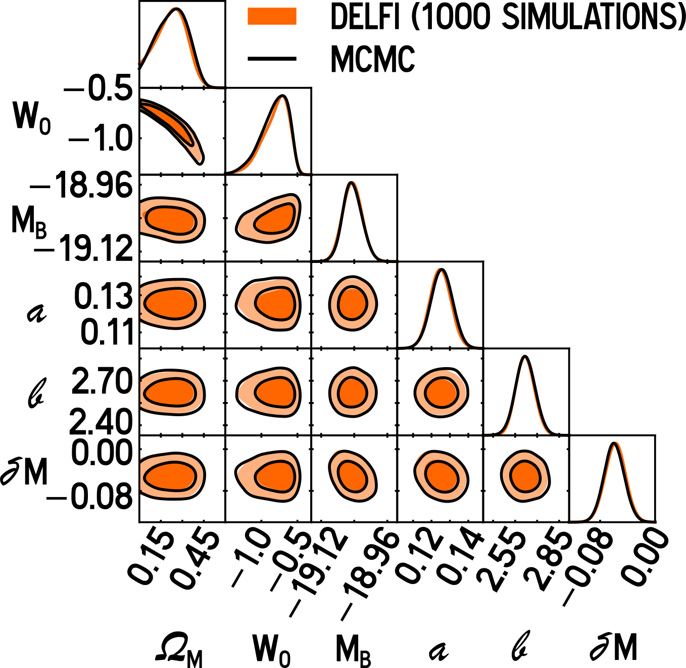
Example 7 : Cosmological parameter inference
(Alsing, Charnock, Feeney and Wandelt 2019)
Beyond loss function stochastic models
- We have so far chosen a loss function which is really the description of the likelihood in our statistical model
We can attempt to fit the posterior with much more complex distributions by inferring the distribution of network weights $p(w|x_\textrm{train},y_\textrm{train},a)\approx q(w|x_\textrm{train},y_\textrm{train},a)$ and calculating
$$p(y|x)=\int_{E_a}\int_{E_w}dadw\,L(y|x,w,a)p(w|x_\textrm{train},y_\textrm{train}, a)p(a)$$This allows for much more abstract distributions, $q(y|x,w,a)\approx P(y|x)$, to be fitted using variational inference.
Note
Current methods described as Bayesian neural networks are not very "Bayesian"
- Distribution is chosen is chosen for the weights and $P(y|x)$ is fitted.
- Quick to train (in general), but there is no certainty about how good the fit is.
In essence there is no difference between a classically trained neural network and what people are calling a Bayesian neural network.
You can have actual Bayesian neural networks where there is no variational assumption on these weights, but these have a lot of other caveats (Charnock, Lavaux, Wandelt, Sarma Boruah, Jasche & Hudson 2020)
Bayes by backprop
Reparameterisation trick
$$\begin{align*} w_i&\sim q(w_i|x_\textrm{train},y_\textrm{train},a)\\ &\equiv\mathbb{N}(\mu_i,\sigma_i)\\ &=\mu_i+\sigma_i\epsilon_i \end{align*}$$where $\epsilon_i\sim\mathbb{N}(0, 1)$ where $i\in[1, n_\textrm{weights}]$.
Calculate $\textrm{ELBO}(q(y|x,w,a))$ and then maximise it using backpropagation for the parameters of the (Gaussian) weight distribution
$$\begin{align*} \mu_i &\leftarrow \mu_i - \eta\left(\partial_{w_i}\textrm{ELBO}(q(y|x,w,a)) + {\partial_{\mu_i}}\textrm{ELBO}(q(y|x,w,a))\right)\\ \sigma_i&\rightarrow \sigma_i-\eta\left(\frac{\epsilon_i}{\sigma}\partial_{w_i}\textrm{ELBO}(q(y|x,w,a)) + {\partial_{\sigma_i}}\textrm{ELBO}(q(y|x,w,a))\right) \end{align*}$$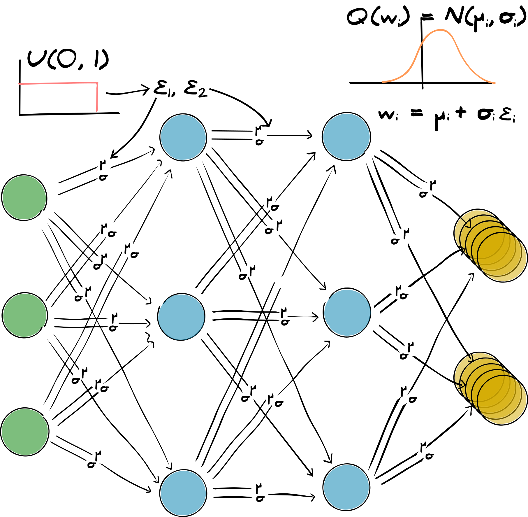
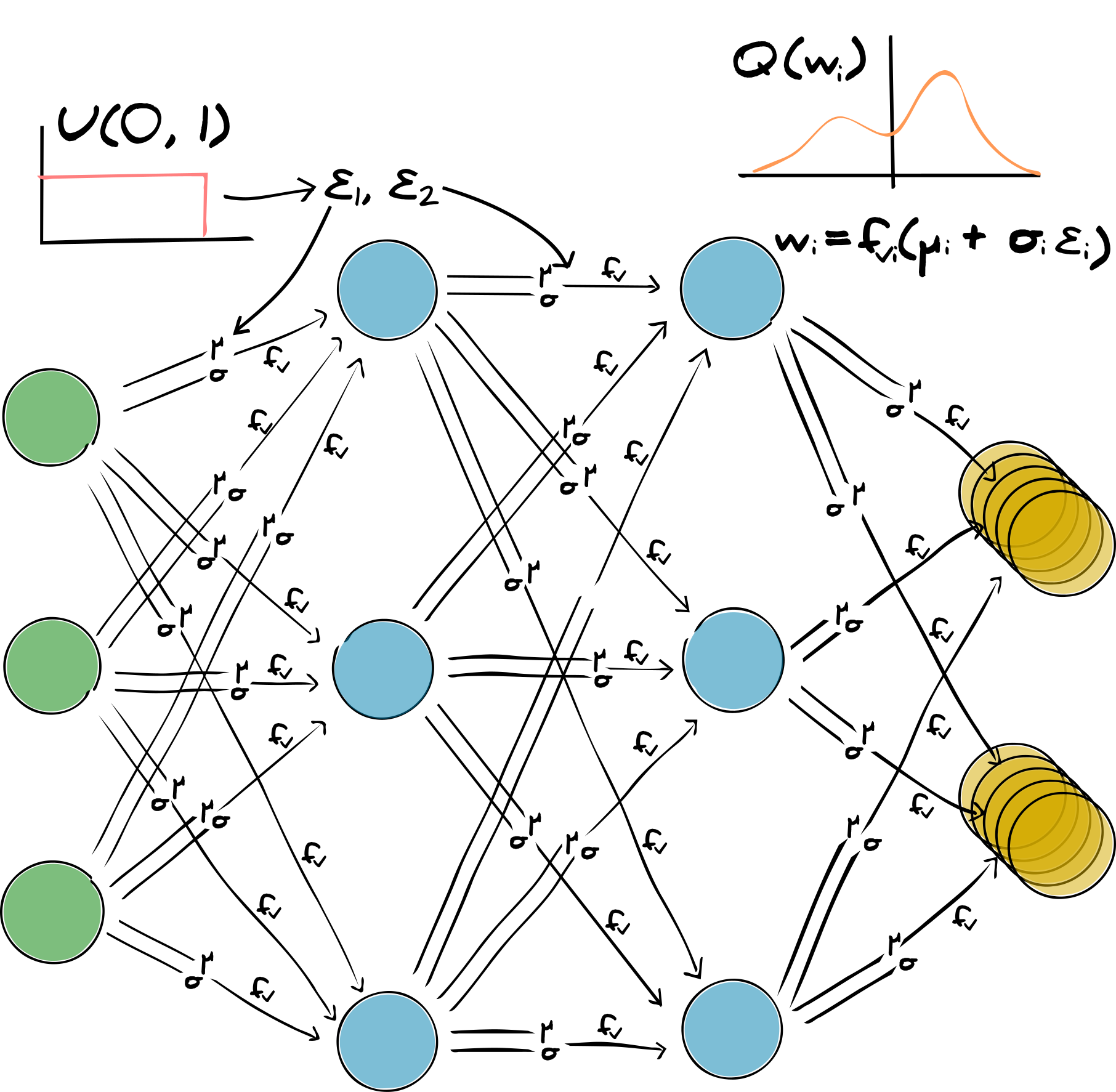
Impracticalities of BbB
$\epsilon$ needs to be drawn for every weight in the network and every element of data in the training set.
This is normally too expensive to actually store using modern hardware or makes computation extremely slow
So we assume just one epsilon for each weight
This is a poor representation of the distribution of parameters and so there is an artificially high variance in the stochastic gradient.
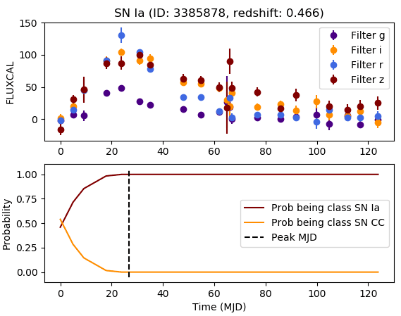
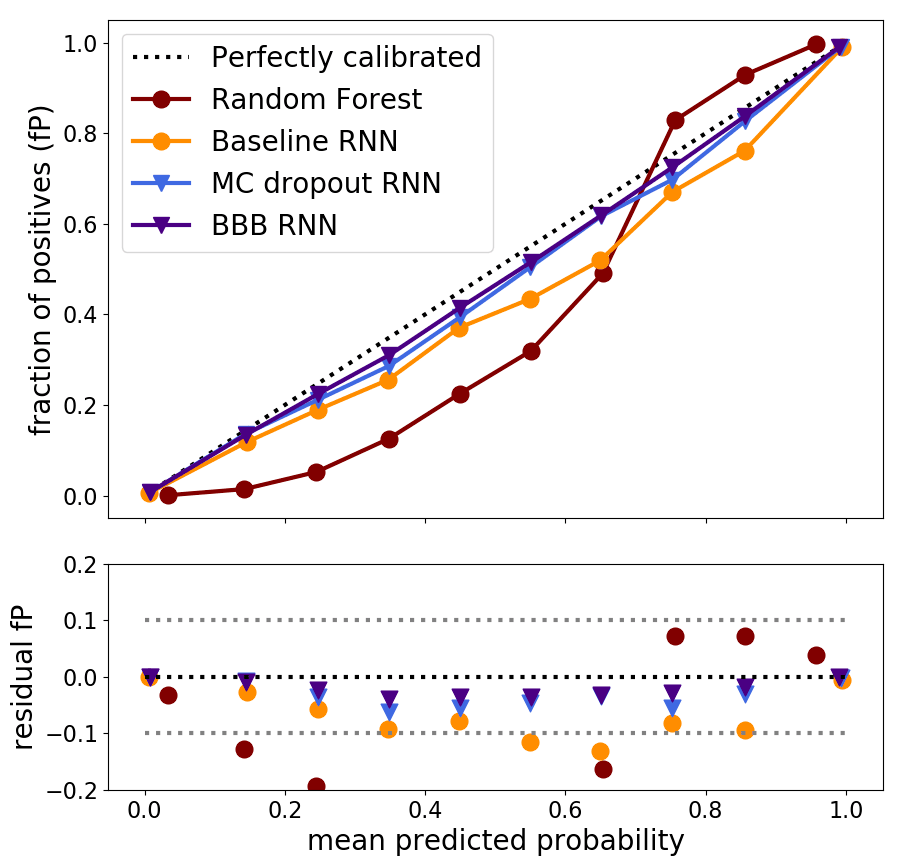
Example 4 : Classification of supernovae type from photometric lightcurves (SuperNNova)
(Möller & Boissiere, 2019)
Recurrent neural network (time series) + Bayes by backprop
Local reparameterisation trick
Model neuron output as $$o_{jn}^l=\sum_{i=1}^{\textrm{dim }l-1}\mu_{ji}^la_{in}^{l-1}+\epsilon_{jn}^l\sqrt{(\sigma_{ji}^l)^2(a_{in}^{l-1})^2}$$
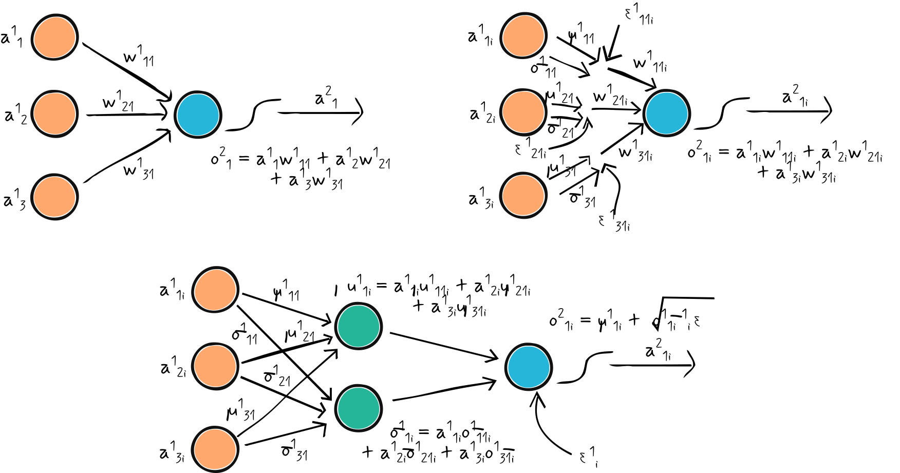
$n_\epsilon$ in BbB $n_\textrm{weights}\times n_\textrm{train}$ $n_\epsilon$ in LRT $n_\textrm{layer outputs}\times n_\textrm{train}$
Whether this is as good of an approximation or not is debatable, its definitely less relatable to the posterior distribution of weights $P(w|x,y,a)$
Variational dropout
Local reparameterisation only works when there is no weight sharing, i.e. it doesn't work for convolutional networks, etc.
We can, however, approximate distributions using multiplicative noise - variational dropout
$$a_{in}^l=\epsilon_{in}^l f(o_{in}^l)$$where $\epsilon_{in}^l\sim\textrm{Dist}(m_{(in)}^{(l)})$ for any distribution.
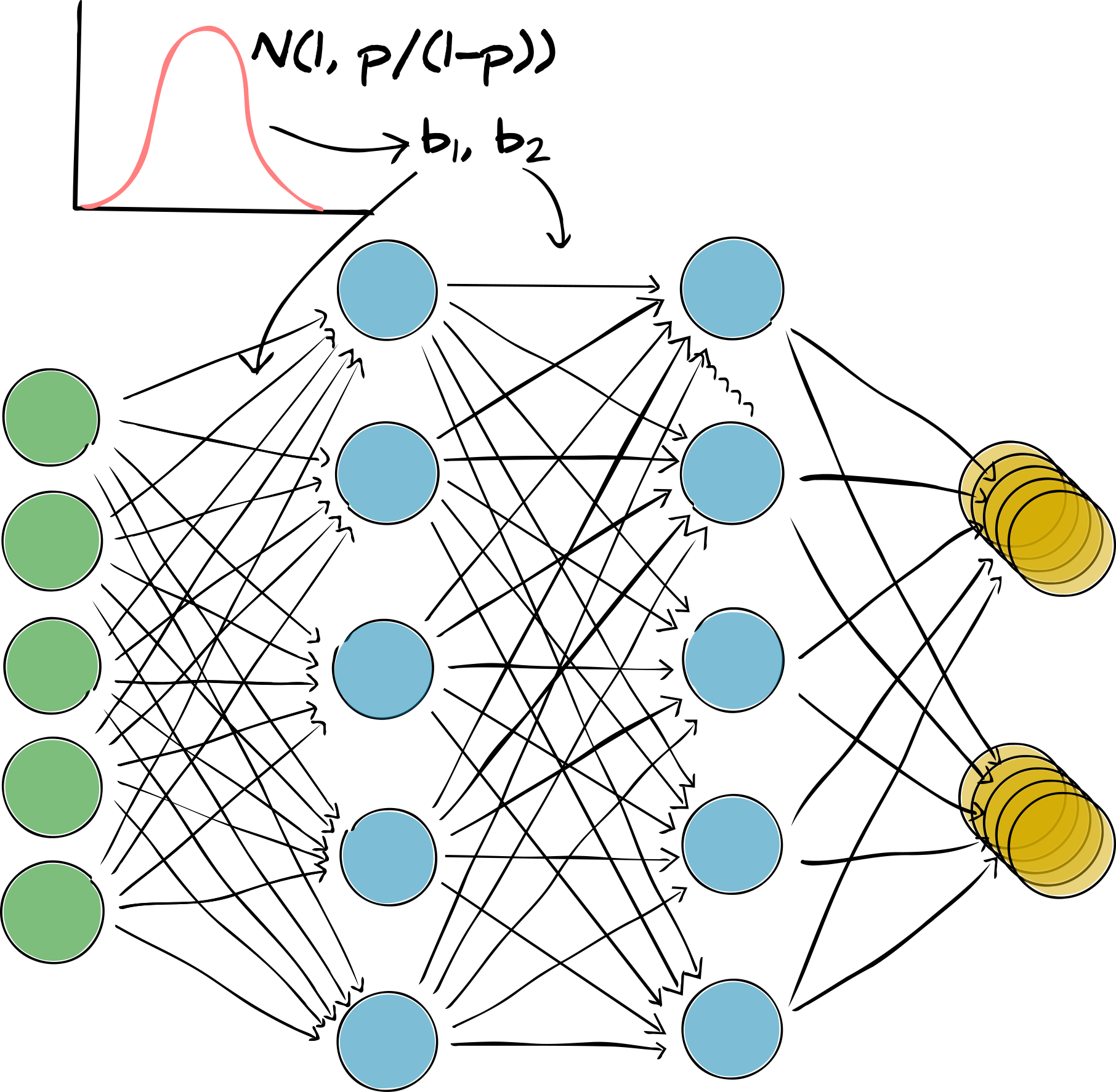
Bernoulli dropout ($\epsilon_{in}^l\sim\textrm{Bernoulli}(b_{(in)}^{(l)})$)
Gaussian dropout ($\epsilon_{in}^l\sim\mathbb{N}(1,b_{(in)}^{(l)})$)
MC Dropout
Train a neural network with dropout (a random dropping of layer outputs) with $\ell_2$ regularisation
equivalent to maximising the ELBO (real VI)
most popular method by far, because of speed and ease of implementation
Variational (and MC) dropout is a very poor representation of $P(w|x,y,a)$ because the distribution of weights isn't considered
- not very Bayesian.
Flipout
Alternative local reparameterisation trick
Symmetric perturbative distribution $w = \mu + \Delta w$ where $\Delta w\sim \textrm{SymDist}$
Draw 2 random vectors $j$ and $k$ of -1 and 1s for each weight and each element in training data
Pseudo-independent weight samples
$$w_{in}=\mu_i+\Delta w_i j_{in}k_{in}$$- Reduces the variance of stochastic gradient by a factor of $1/n_\textrm{elems}$
- Best results at the moment from variational inference.
Note that this might be a bad estimate of $P(w|x,y,a)$ because we have to assume that it is unimodal and symmetric - which is almost certainly not a good approximation of $P(w|x,y,a)$.