Machine learning and statistics in astronomy and cosmology
Tom Charnock
Institut d'Astrophysique de Paris
Slides available at presentations.charnock.fr/MPP



Overview
Some terminology
Statistical modeling
Machine learning to accelerate science
- targeting rare objects in photometric surveys
Neural networks in Bayesian analysis
- agnostic inference of the halo mass distribution function
Likelihood-free inference
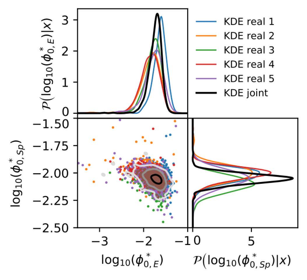
- neural compression for inference of galatic population models
A little terminology
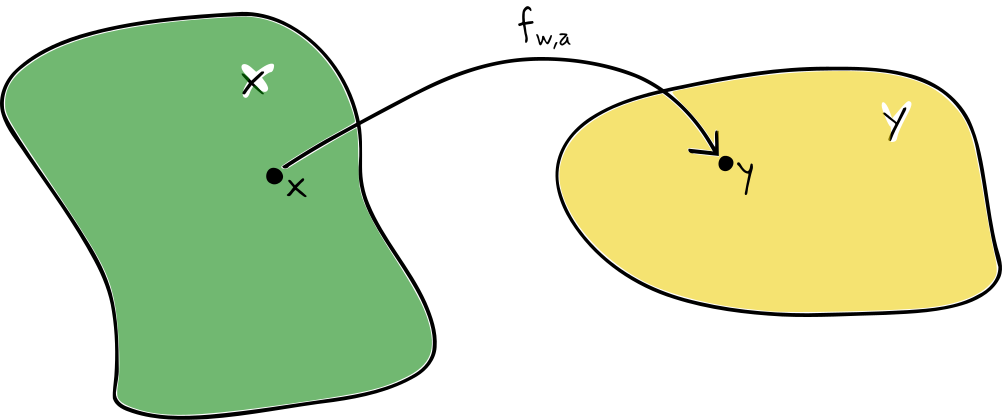
Neural networks - parameterisable functions $\mathscr{f}_{w,a}:x\in\mathcal{X}\mapsto y\in\mathcal{Y}$
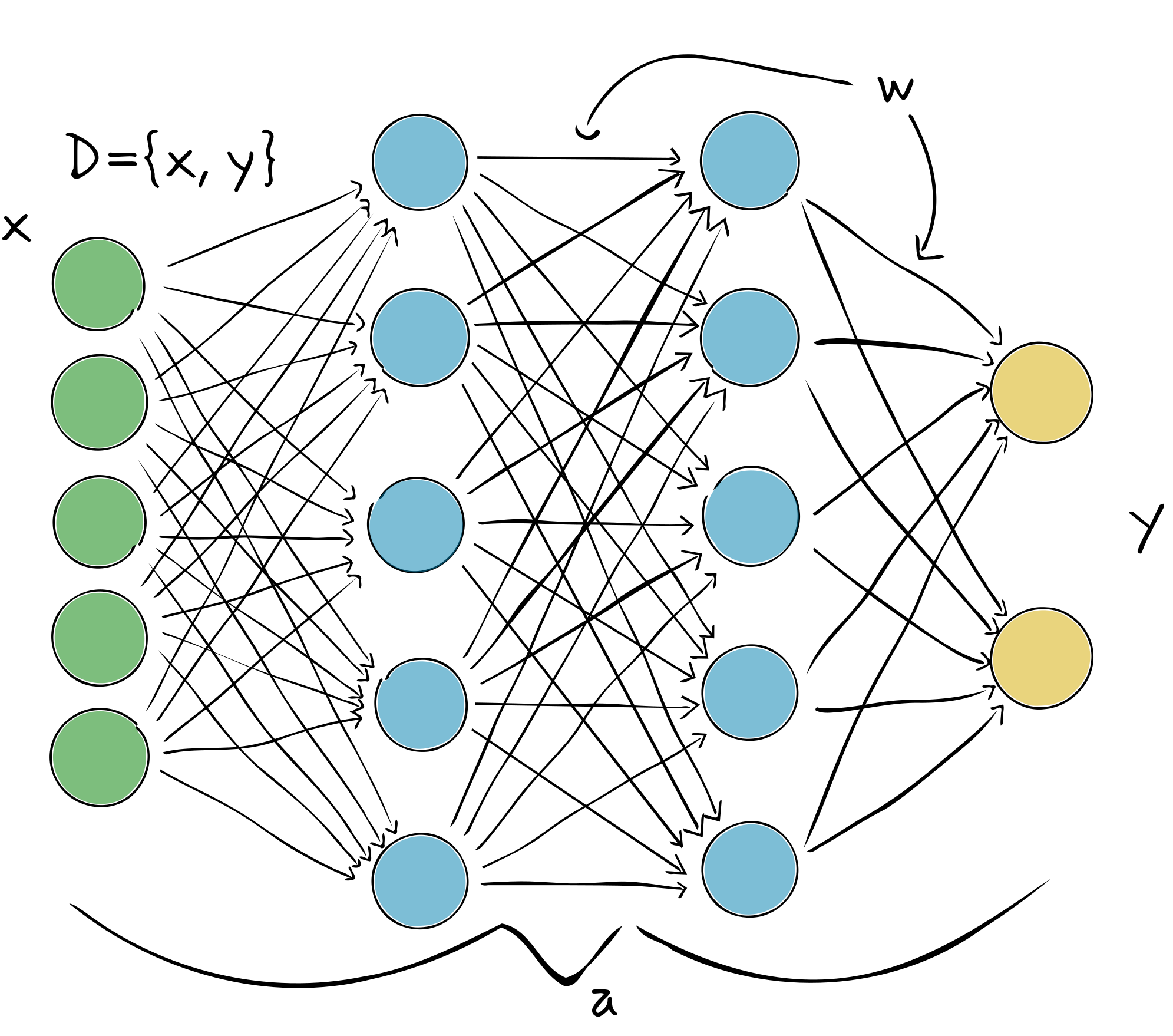
Stacks of non-linear activated weighted sums - \\(\displaystyle n_j^l = \phi\left(\sum_iw_{ji}n^{l-1}_i+b_j\right)\\)
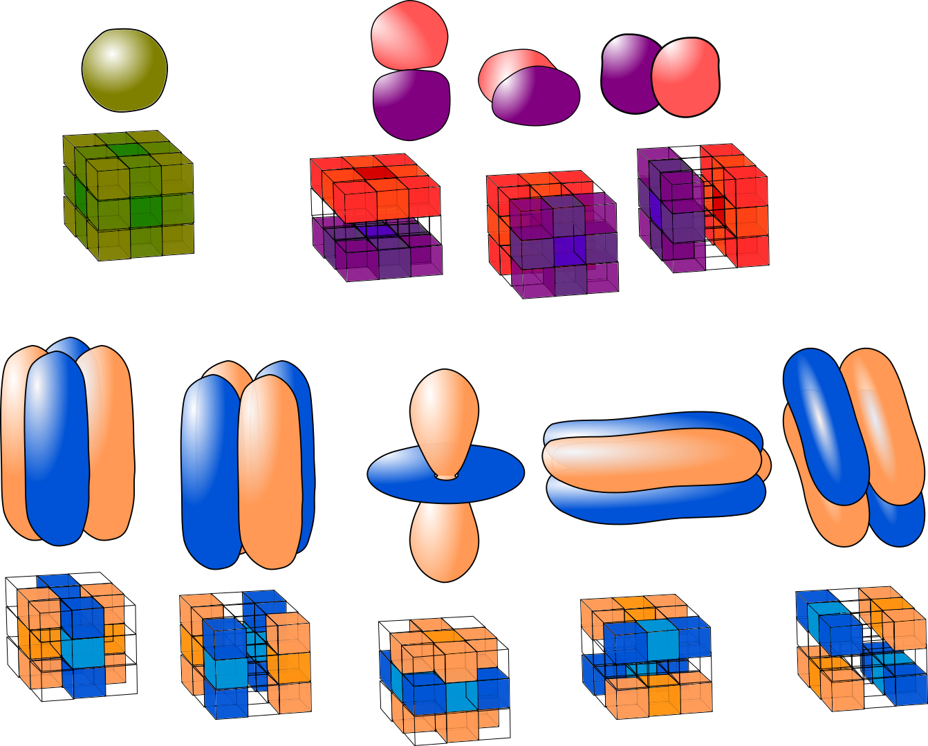
Architectures (and their relation to physics)
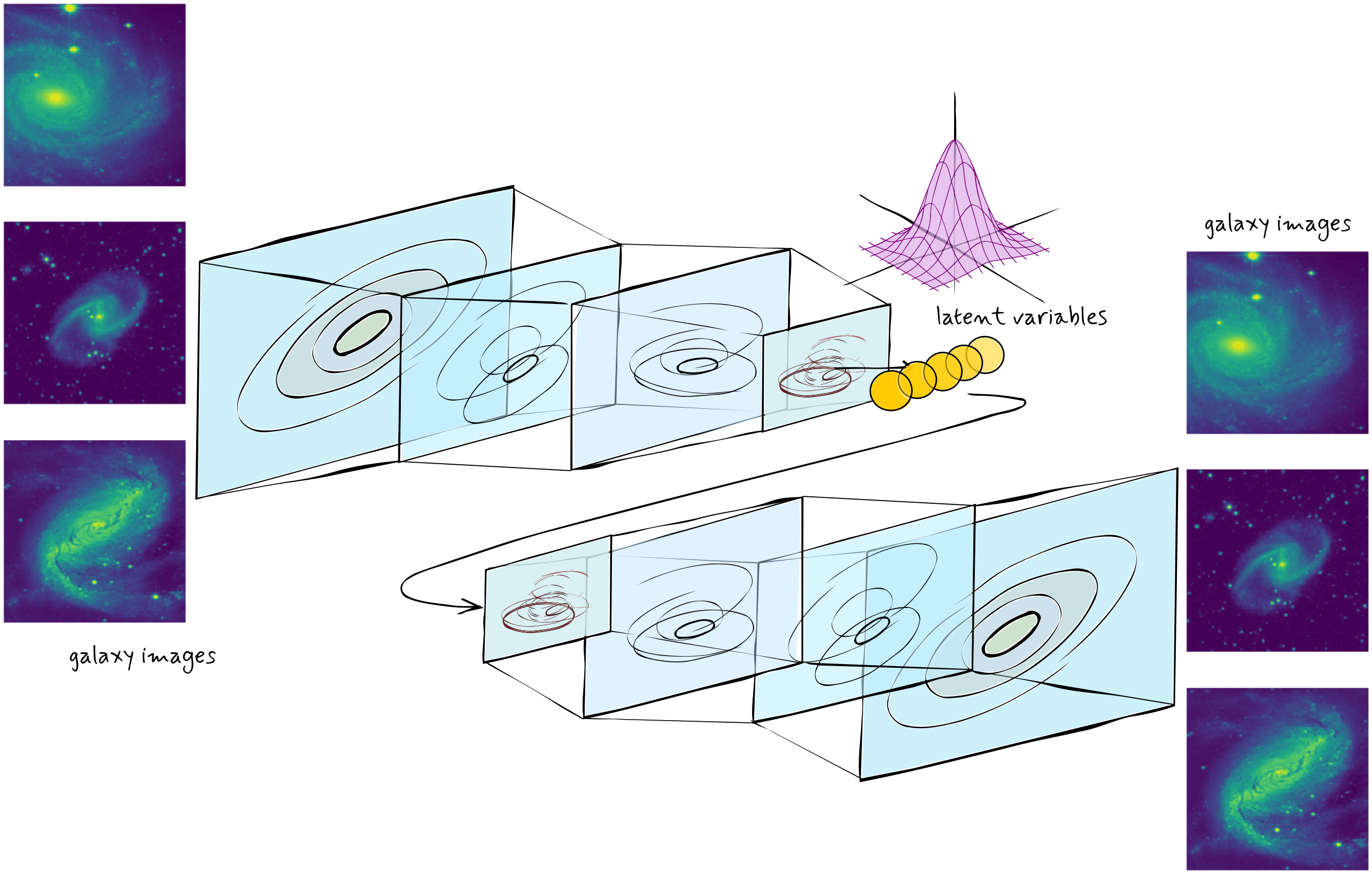
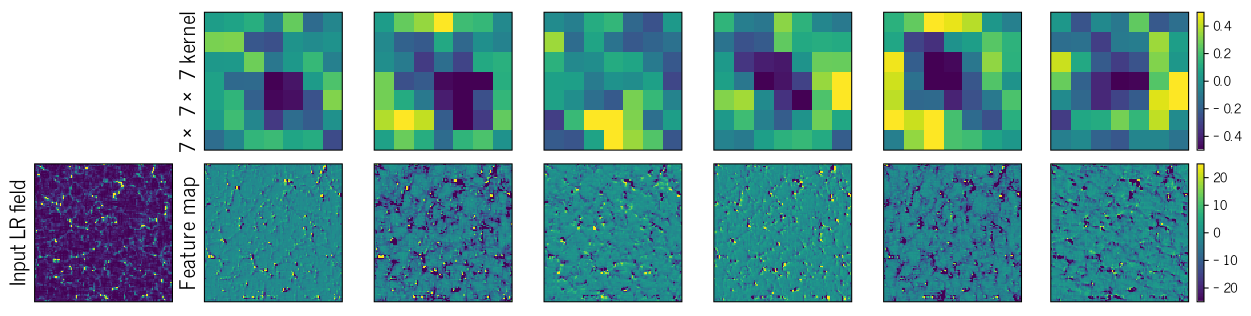
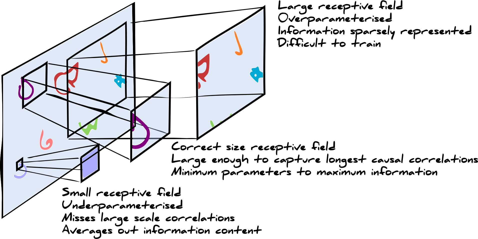
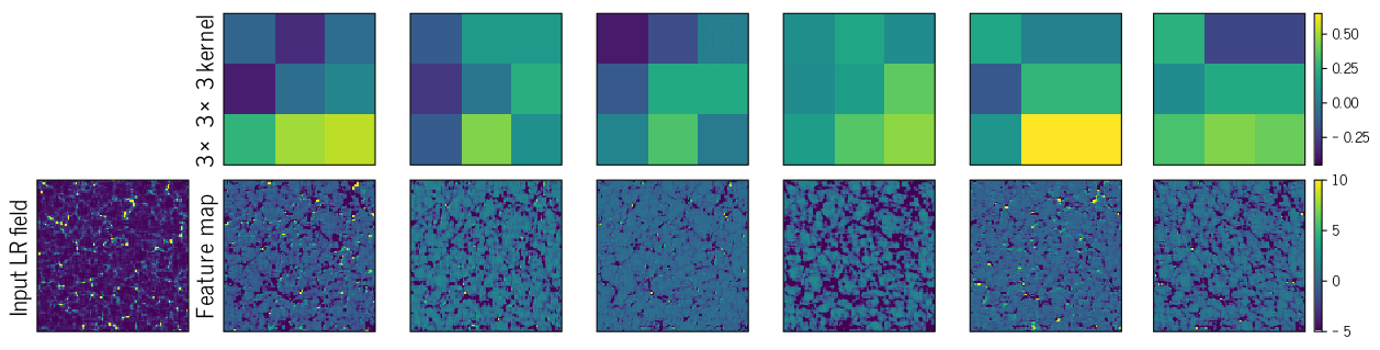
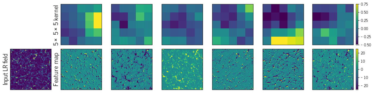
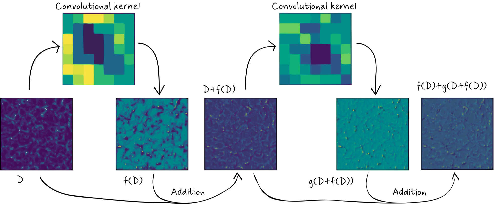
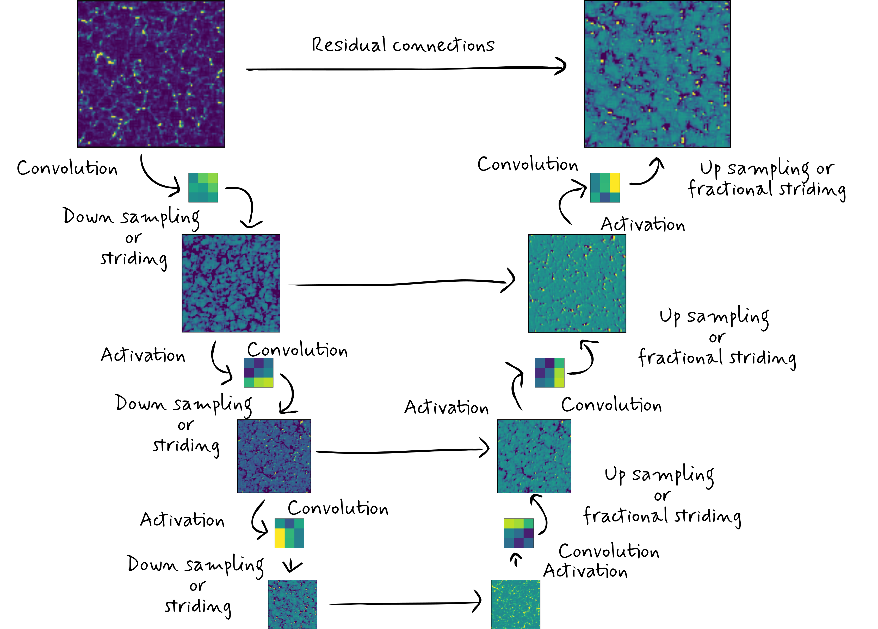
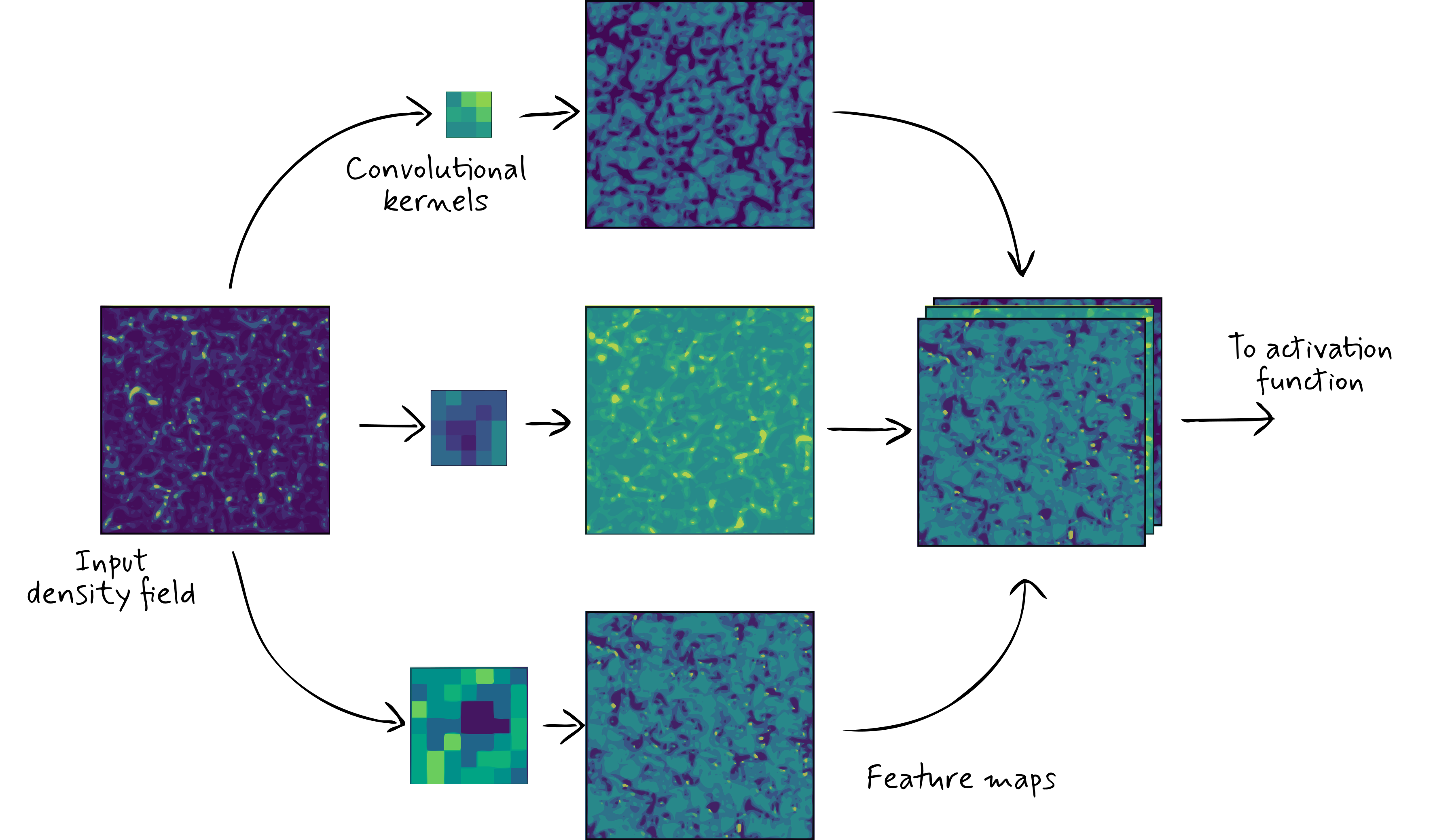
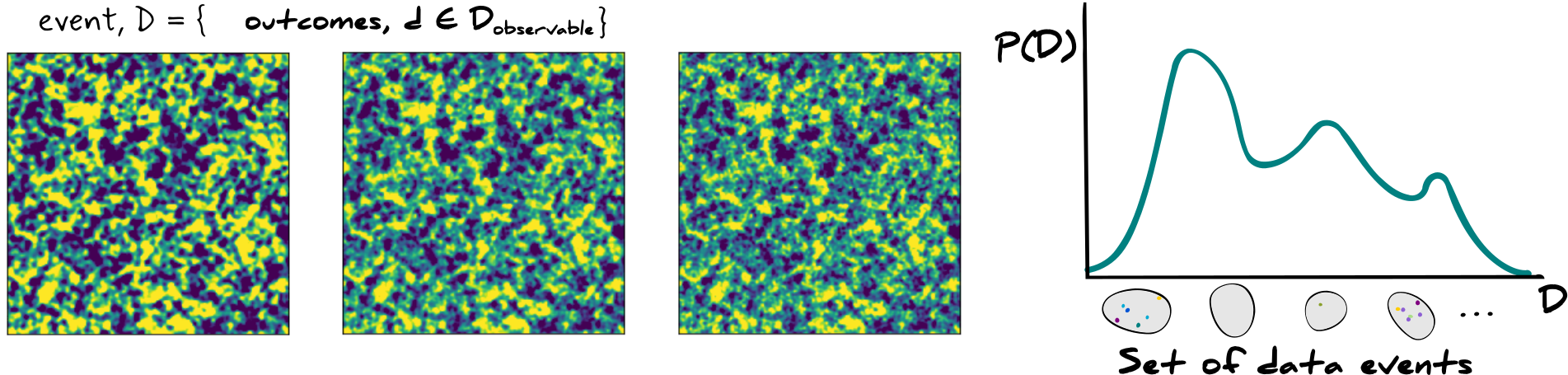
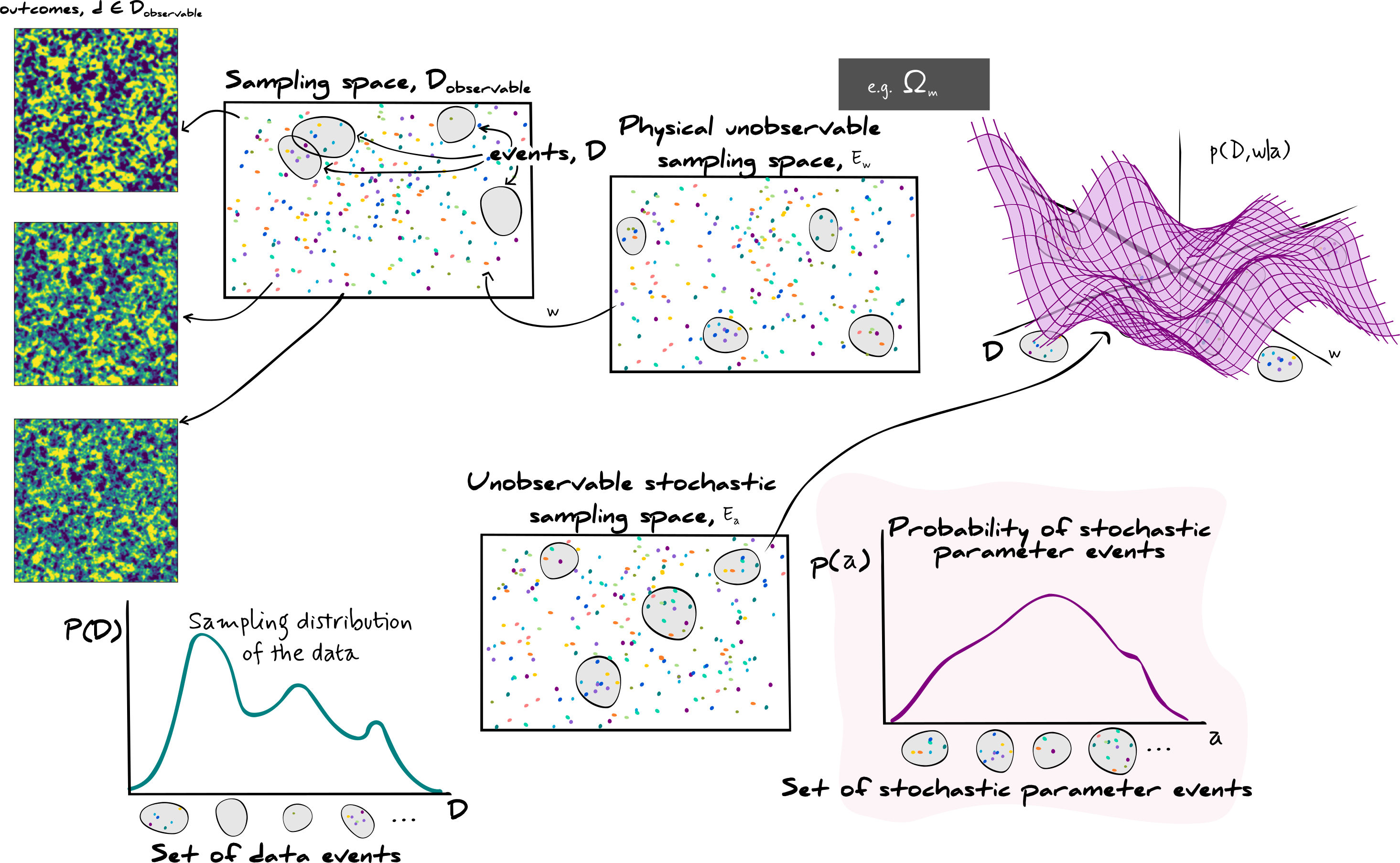
Why do we even care...
we should be talking about neural networks!
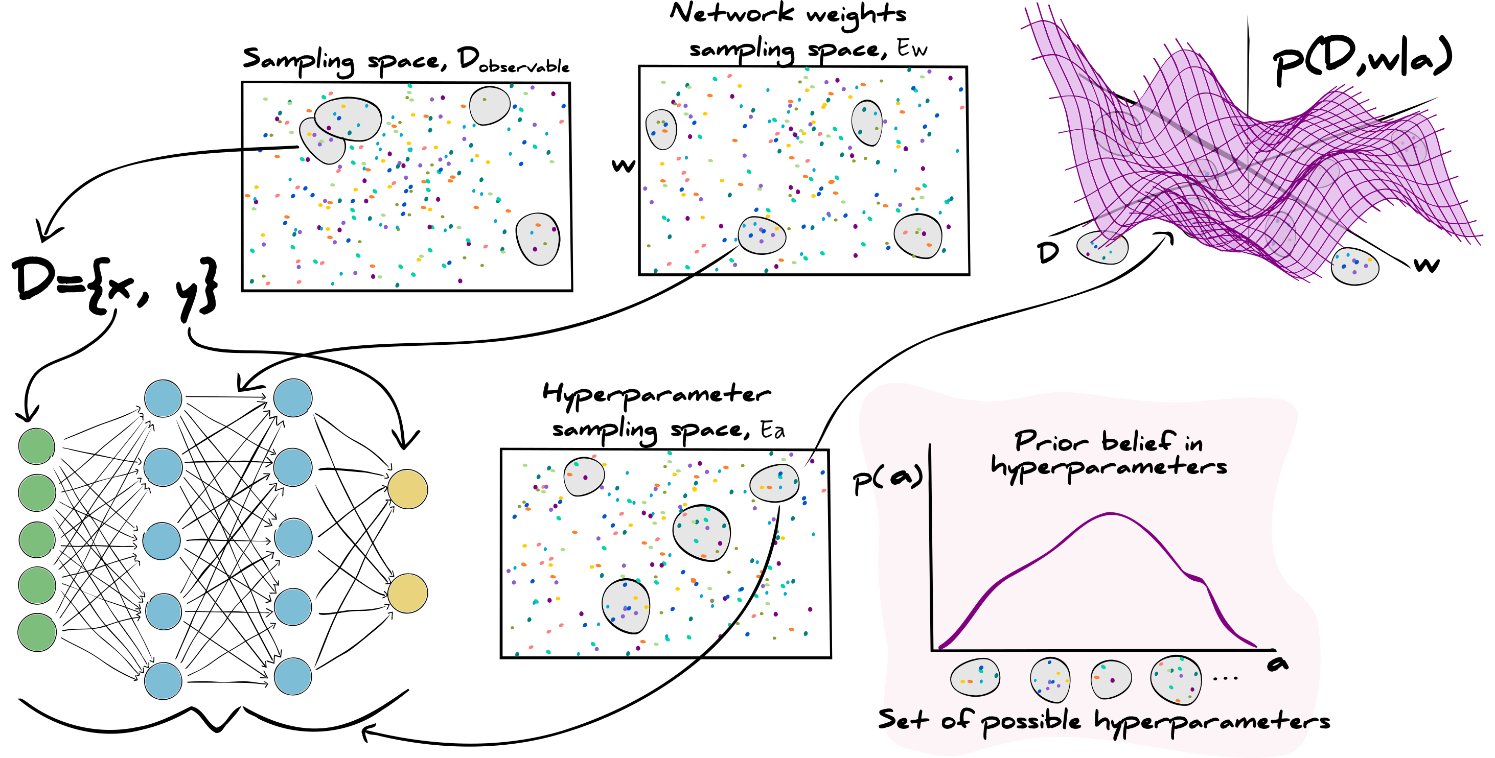
How can we do that?
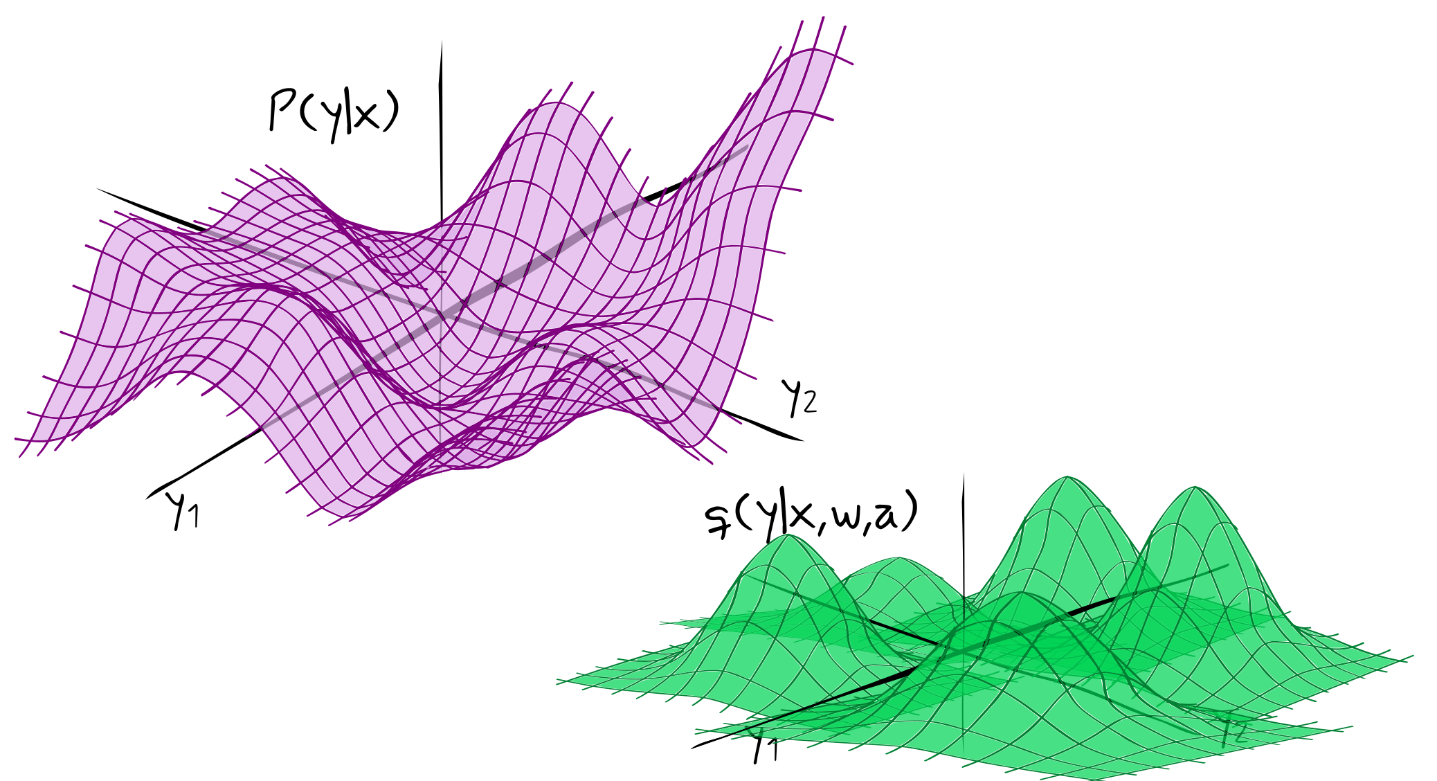
Relative entropy
A measurement of the information loss by approximating a distribution, $P(y|x)$, with some other distribution, $q(y|x,w,a)$.
$$\mathbb{D}[P(y|x)||q(y|x,w,a)]=\int_{E_y}dyP(y|x)\ln\frac{P(y|x)}{q(y|x,w,a)}$$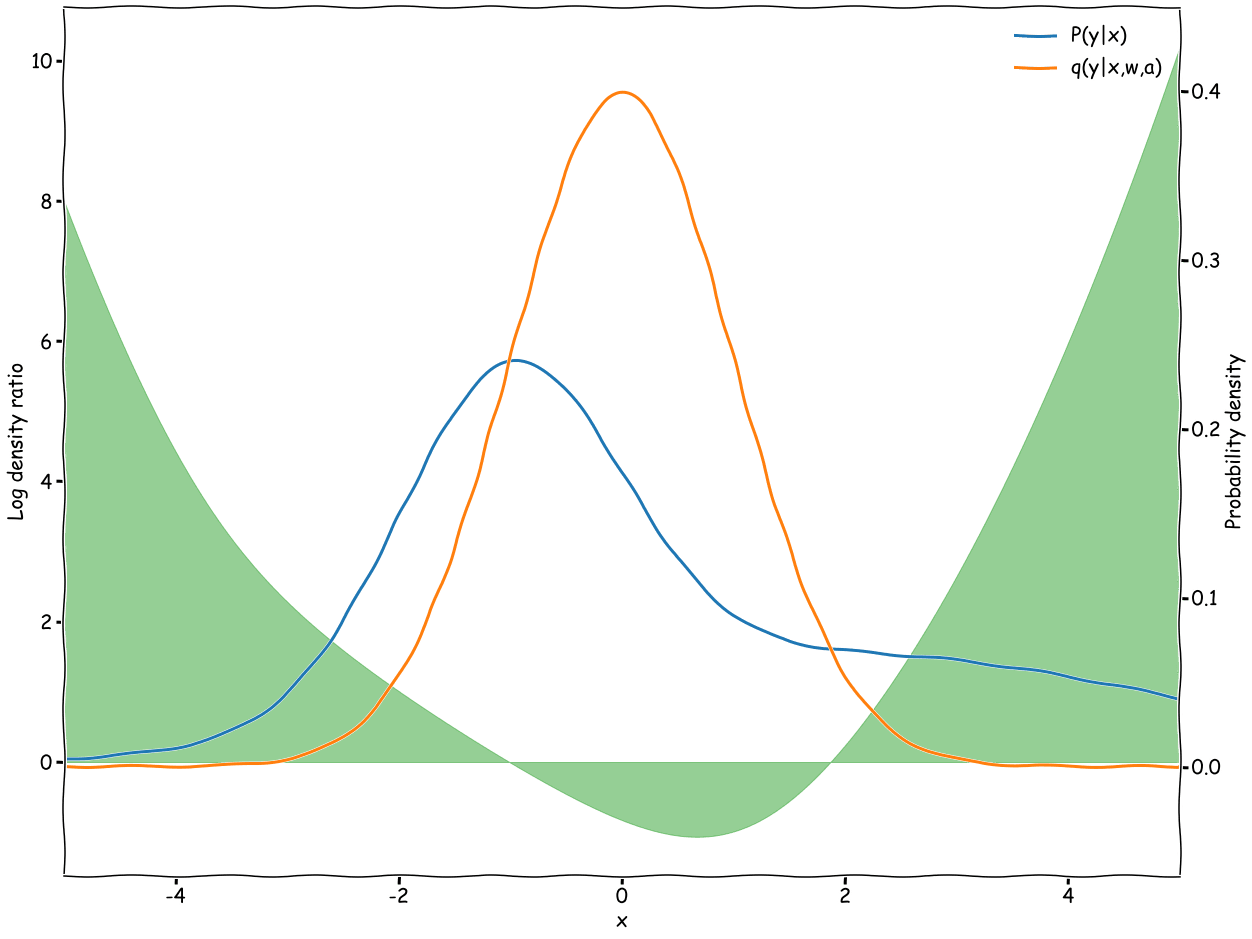
Identical distributions
$$\mathbb{D}[P(y|x)||q(y|x,w,a)]=0\textrm{ means }P(y|x)=q(y|x,w,a)$$Different distributions
$$\mathbb{D}[P(y|x)||q(y|x,w,a)]>0\textrm{ means }P(y|x)\ne q(y|x,w,a)$$Non-symmetric (not a real distance metric)
$$\mathbb{D}[P(y|x)||q(y|x,w,a)]\ne[\mathbb{D}[q(y|x,w,a)||P(y|x)]$$What is the relative entropy?
$$\begin{align*} \mathbb{D}[P(y|x)||q(y|x,w,a)]&=\int_{E_y}dyP(y|x)\ln\frac{P(y|x)}{q(y|x,w,a)}\\ &=-\int_{E_y}dyP(y|x)\ln q(y|x,w,a)+\int_{E_y}dyP(y|x)\ln P(y|x) \end{align*}$$Entropy of $P(y|x)$
Cross entropy between $P(y|x)$ and $q(y|x,w,a)$
The cross-entropy measures the average number of bits of information needed to tell that an event is drawn from $q(y|x,w,a)$ rather than $P(y|x)$
We don't actually know $P(x,y)$ - that's what we want to model
We just have distribution of observed samples, $P(\{x,y\}_\textrm{train})$, made up of
$$\{x_i,y_i\sim P(x,y)|i\in[1,n_\textrm{train}]\}$$(hopefully very close to $\approx P(x,y)$)
Using this sampling distribution we can rewrite the relative entropy as
$$\mathbb{D}[P(y|x)||q(y|x,w,a)]=-\sum_{i=1}^{n_\textrm{train}}P(y_i|x_i)\ln q(y_i|x_i,w,a)+\sum_{i=1}^{n_\textrm{train}}P(y_i|x_i)\ln P(y_i|x_i)$$By minimising the relative entropy we can attempt to bring $q(y|x,w,a)$ close to $P(y|x)$
(or at least $P(y_\textrm{train}|x_\textrm{train})$).
Entropy term, $P(y|x)$ is independent of $w$, so optimising the parameters of $q(y|x,w,a)$ is equivalent to minimising the cross-entropy
$$\begin{align*} \widehat{w}&=\underset{w\in E_w}{\textrm{arg min}}\,\mathbb{D}[P(y|x)||q(y|x,w,a)]\\ &=\underset{w\in E_w}{\textrm{arg min}}\,-\sum_{i=1}^{n_\textrm{train}}P(y_i|x_i)\ln q(y_i|x_i,w,a) \end{align*}$$How can we calculate the cross entropy?
The likelihood of a training set is
- how often each event, $y_i$, in the training set occurs (or the probability, $P(y_\textrm{train}|x_\textrm{train})$)
- the estimation of the probability using the likelihood, $q(y_i|x_i,w,a)$, for every event
Taking the logarithm (divided by the number of training samples) gives
$$\begin{align*} \frac{1}{n_\textrm{train}}\ln L(y_\textrm{train}|x_\textrm{train})&=\frac{1}{n_\textrm{train}}\ln\prod_{i=1}^{n_\textrm{train}}q(y_i|x_i,w,a)^{n_\textrm{train}P(y_i|x_i)}\\ &=\sum_{i=1}^{n_\textrm{train}}P(y_i|x_i)q(y_i|x_i,w,a) \end{align*}$$Minimising the cross-entropy is equivalent to maximising the logarithm of the likelihood!
Maximum-likelihood estimation!
$$\widehat{w}=\underset{w\in E_w}{\textrm{arg min}}-\ln L(y_\textrm{train}|x_\textrm{train})$$
Equivalent to minimising the relative entropy and bringing $q(y|x,w,a)$ as close to $P(y|x)$ as possible.
(This comes with all the pitfalls that are prevalent with MLE)
What are the outputs of neural networks then?
where $\gamma$ are the parameters of our distribution describing the probability of our data
$$q(y|x,w,a) \propto \textrm{Loss}(\gamma, y)$$Mean square error: $\gamma$ is the mean of a unit variance Gaussian likelihood for $y$
Softmax (sigmoid) output: $\gamma$ is the probability of the occurance of $y$ in a Bernoulli distribution
Absolute error: $\gamma$ is the diversity of a zero centred Laplace distribution for the probability of $y$
Are these models any good?
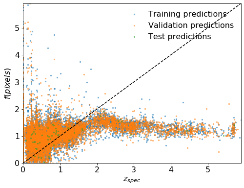
No...
Neural networks are highly complex functions with no specific reason to be globally smooth.
The $\gamma$ describing targets $y$ or $y'$ from inputs $x$ and $x'$ have no reason to be consistent, even if $x$ and $x'$ are infinitessimally close.
Very difficult to make a predictive statement about how likely is any $y$ when given a neural network
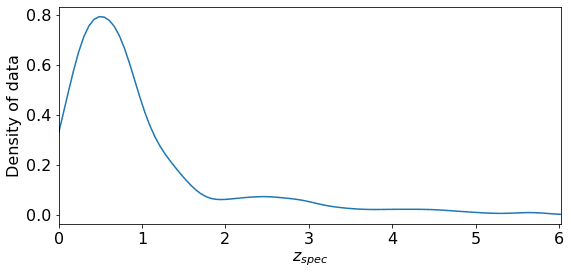
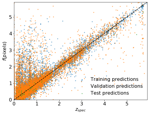
Distribution of spectroscopic redshifts in a spectroscopic catalogue
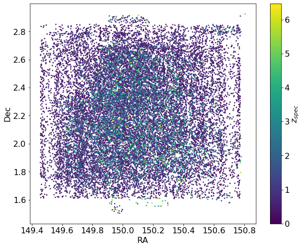
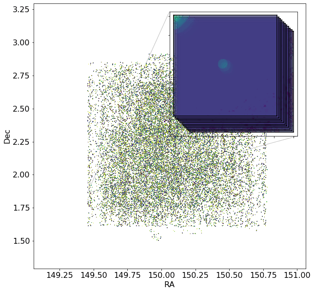
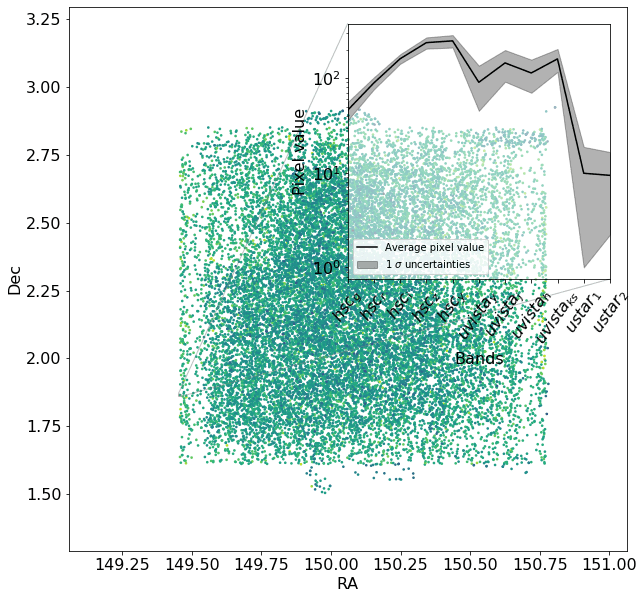
Select patches/pixels from COSMOS2020 by RA and Dec
HSC $g$, $r$, $i$, $z$, $y$
ULTRAVista $y$, $h$, $j$, $ks$
CFHT u* 1, 2
Error model for pixel values, $\textsf{pix}$:
$$\begin{align*} \textsf{pix}_i &\sim P(\textsf{pix}|\{\text{CCD read out}\}_i)\\ & \approx \mathcal{N}(\boldsymbol{\mu}_{\textsf{pix},i},\boldsymbol{\Sigma}_{\textsf{pix},i}) \end{align*}$$
According to data, there should always be more likely to have objects with redshifts between 0 and 1
The first fits the data better, but we can't see it because the mean and mode are not good measures...
If we want a flat prior over physical properties, we need to reweight the effect of the data
The mean of the data distribution
(for a single Gaussian)
The mean of the reweighted distribution
(for a single Gaussian)
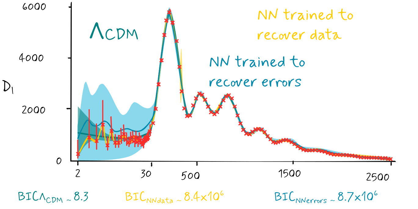
When comparing different models we tend to use statistics such as the Bayesian evidence ratio
$\displaystyle B = (\ln)\frac{p(D|a_2)}{p(D|a_1)}$
As physicists we prefer some quantification of simplicity (Occam's razor)
- $BIC = k\ln n - 2\ln L(D|w^*, a)$
- $AIC = 2k - 2\ln L(D|w^*, a)$
i.e. we prefer ΛCDM over a polynomial fit with tons of parameters and therefore fits the data perfectly, but is not predictive.
Neural networks will always lose at model comparison stage
Although predictions can be validated using a test set there is no physical principle which will tell us the general behaviour for any new piece of data... we just have to hope!
Is there any hope for using machine learning?
Of course there is...
We can see that neural networks are able to extract ridiculously large amounts of information directly from the data.
We just need to use the extracted information in a way that does not depend on the neural network as a model or only use them in the case when the model isn't important for scientific results...
Machine learning accelerated science
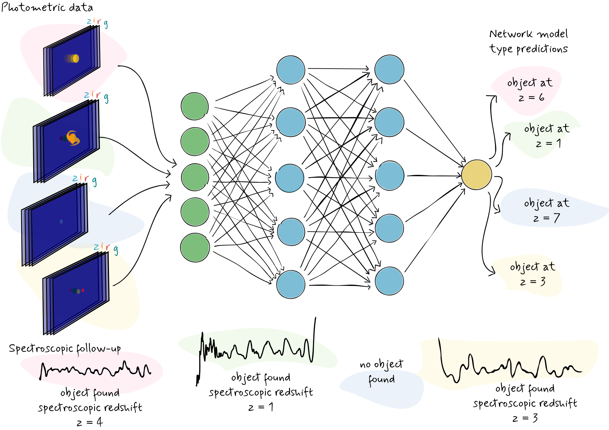
How do we choose where to target follow-up observations?
Modelling the probability of redshifts given the existance of objects
Flexible enough to model the fact that the distribution of objects is skewed
Simple enough that we can perform analytical integrals
Mixture of Gaussians
$$P_\mathscr{w}(z|\textsf{obj}_i, \textsf{pix}_i) = \sum_k \alpha_k(\textsf{pix}_i, \mathscr{w})\hskip0.1em\mathcal{N}\hskip-0.25em\left(\mu_k(\textsf{pix}_i, \mathscr{w}), \sigma_k(\textsf{pix}_i, \mathscr{w})\right)$$Targetting rare objects
Calculate the marginal distribution for the probability of objects given particular properties, i.e.
High redshift objects, i.e. $z > 6$
$$P_\mathscr{w}(\textsf{obj}|\textsf{pix}_i, z>6)=\int_6^\infty dz \,P_\mathscr{w}(\textsf{obj}|z, \textsf{pix}_i)P_\mathscr{w}(z|\textsf{pix}_i)$$Naïvely seach for maximal probability of objects
$$\hat{i} = \underset{i\in\textrm{Survey}}{\textrm{argmax}}~P_\mathscr{w}(\textsf{obj}|\textsf{pix}_i, z>6)$$Targetting objects by maximising the probability of particular properties over entire field
$$\hat{i} = \underset{i\in\textrm{Survey}}{\textrm{argmax}}~P_\mathscr{w}(\textsf{obj}, z|\textsf{pix}_i)$$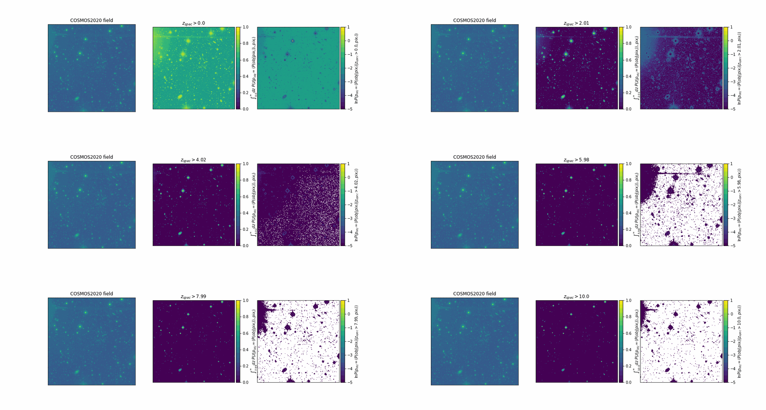
A way to find rare objects
Neural networks using in a Bayesian setting
(Charnock, Lavaux, Wandelt, Sarma Boruah, Jasche and Hudson 2020)
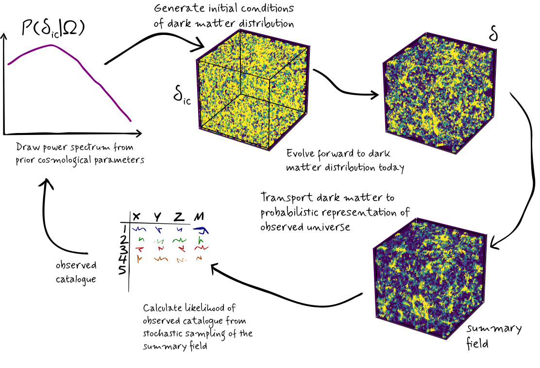
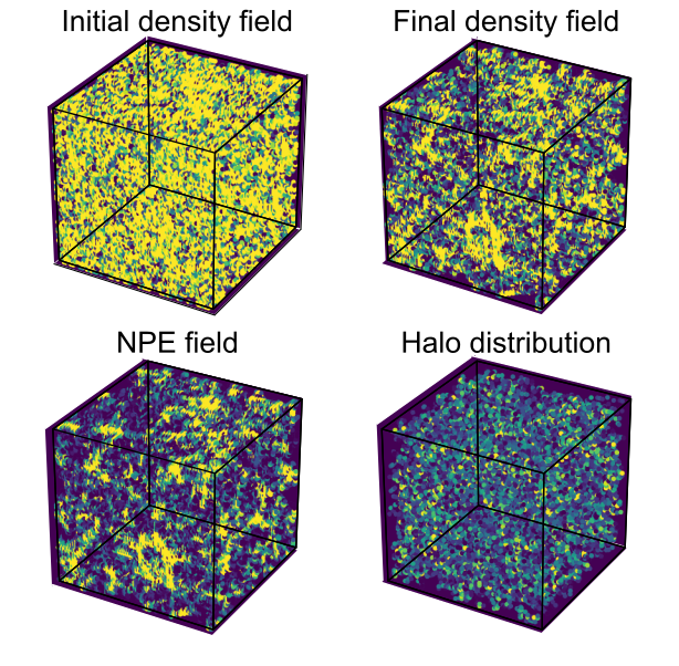
Inferring cosmological parameters and initial conditions of simulations from noisy (horrible) data
- Forward model all understood physics
- Make abstract function (NN) made from physically motivated architecture choice
- Use high dimensional Markov methods to sample physical properties AND neural network parameters
Not deep learning anymore - we're just benefitting from the differentiable frameworks and doing old-school* physics 😉
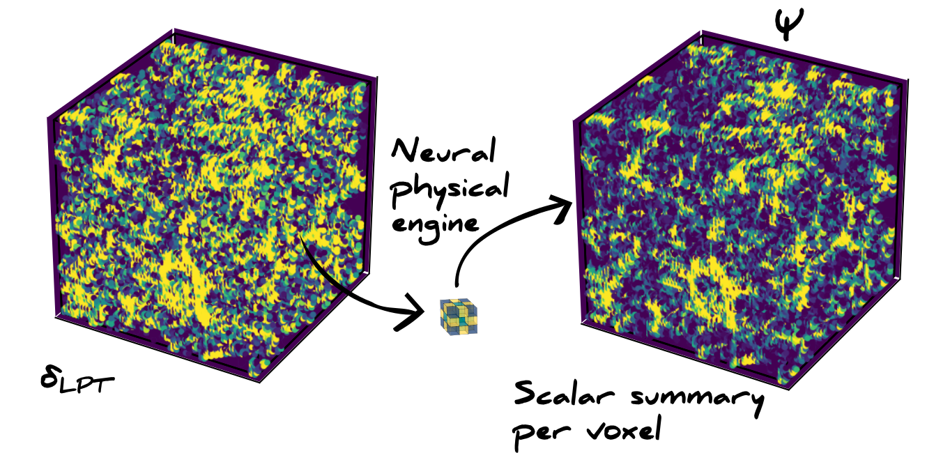
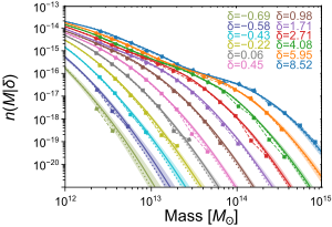
A functional describing the distribution of halos in voxels
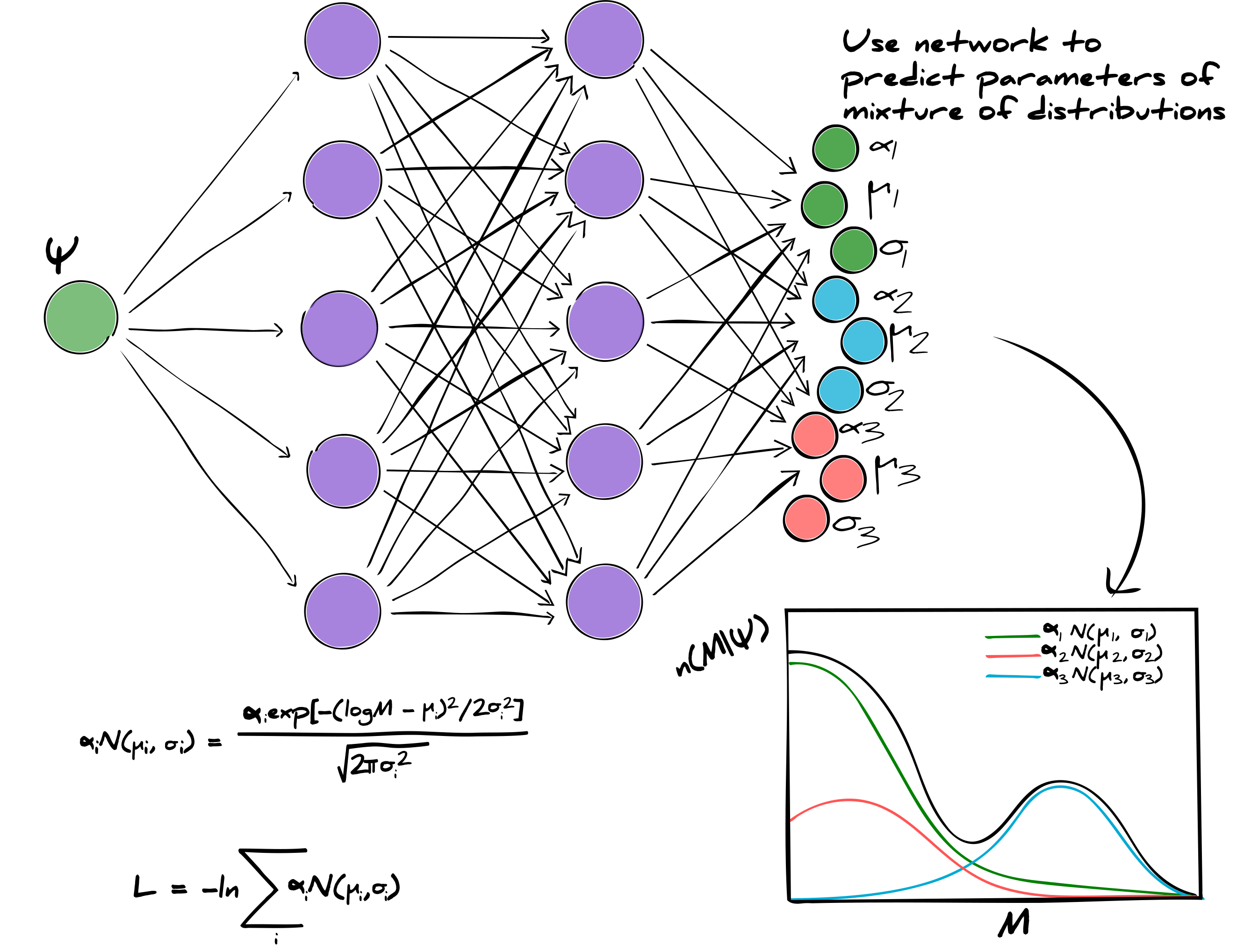
And a likelihood describing how likely a catalogue could be generated from such a halo mass distribution function
$$\begin{align*} {\Tiny\mathcal{L} =}&{\Tiny \sum_{j\in\textrm{catalogue}}\log\left[\sum_i^N\frac{\alpha_{i,j}}{\sqrt{2\pi\sigma_{i,j}^2}}\exp\left[-\frac{\left(\log(M_j) - \mu_{i,j}\right)^2}{2\sigma_{i,j}^2}\right]\right]}\\ &{\Tiny - V\sum_{j\in\textrm{voxels},i=1}^N\frac{\alpha_{i,j}}{2}\exp\left[\frac{\sigma_{i,j}^2}{2}\right]\textrm{erfc}\left[\frac{\log\left(M_\textrm{th}\right) - \mu_{i,j} - \sigma_{i,j}^2}{\sqrt{2\sigma_{i,j}^2}}\right].} \end{align*}$$Use high order Hamiltonian Monte Carlo sampling to infer:
The cosmological parameters which give rise to a realistic power spectrum
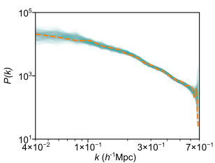
The initial conditions which could give rise to the distribution of halos we see
The Markov chain of parameter values of the neural network
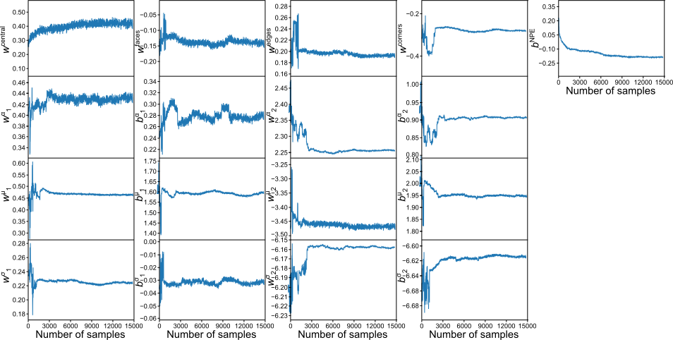
(We can marginalise out these parameters to ignore the effect of the network on the overall physics)
And therefore the possible values of the halo mass distribution function
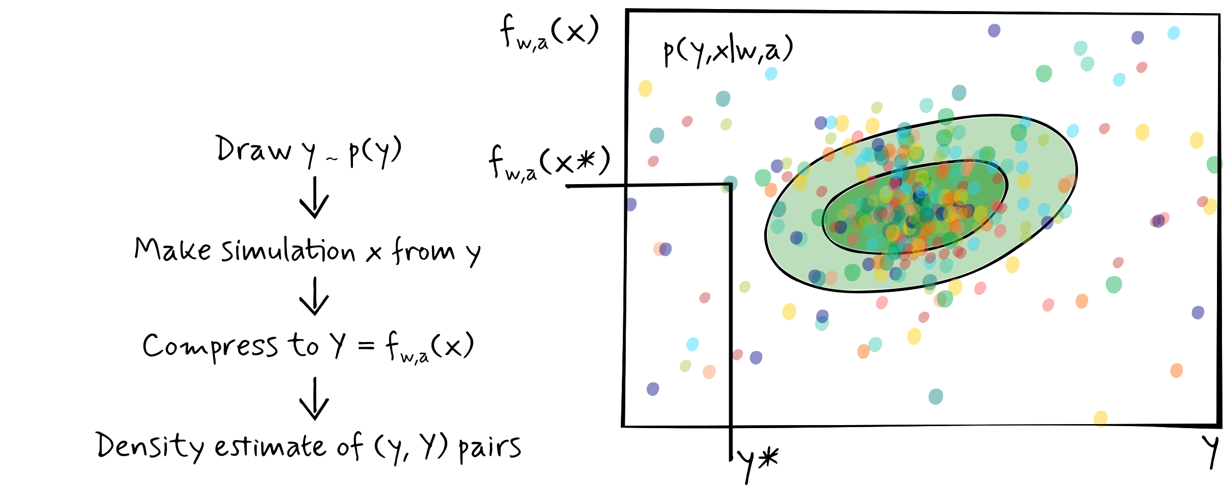
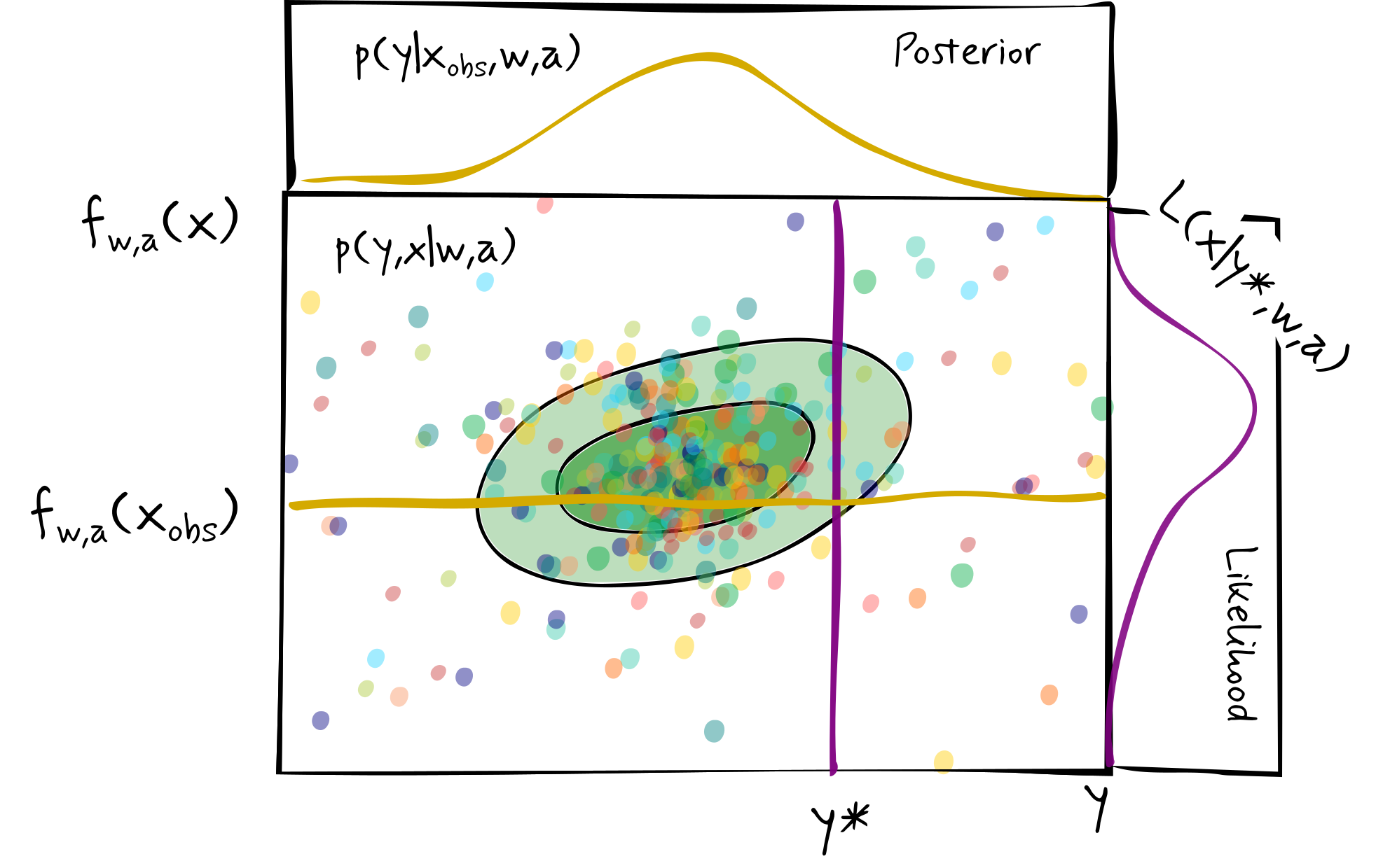
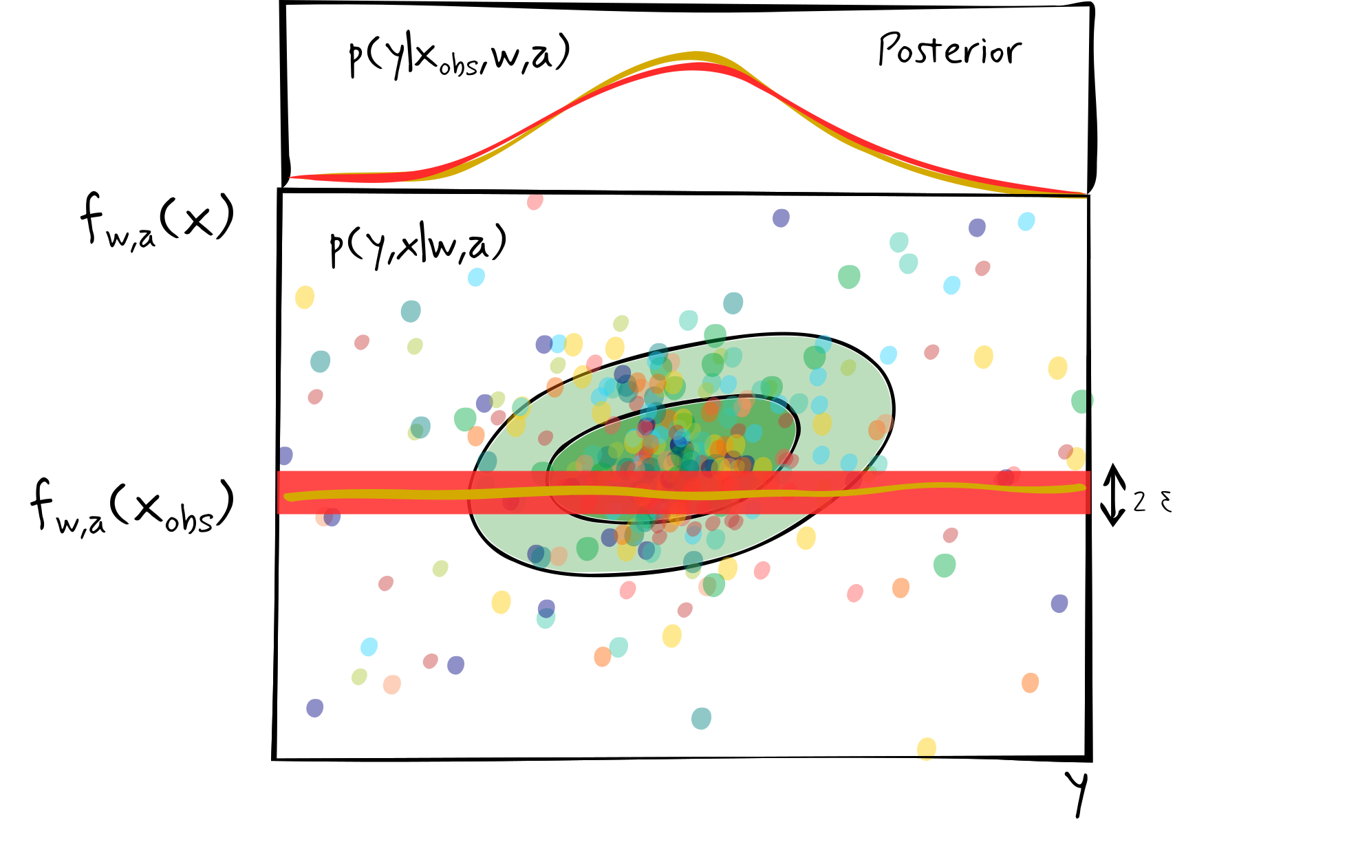
Approximate Bayesian computation (ABC)
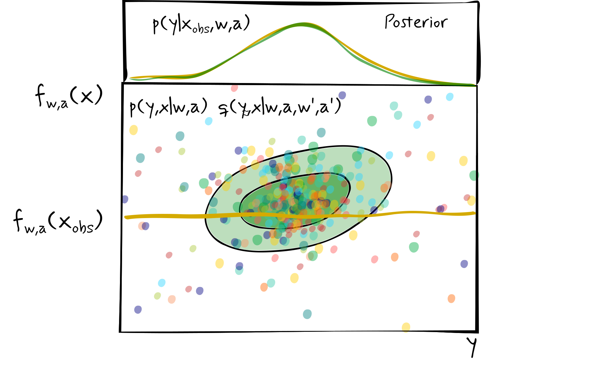
Density estimate likelihood-free inference (DELFI)
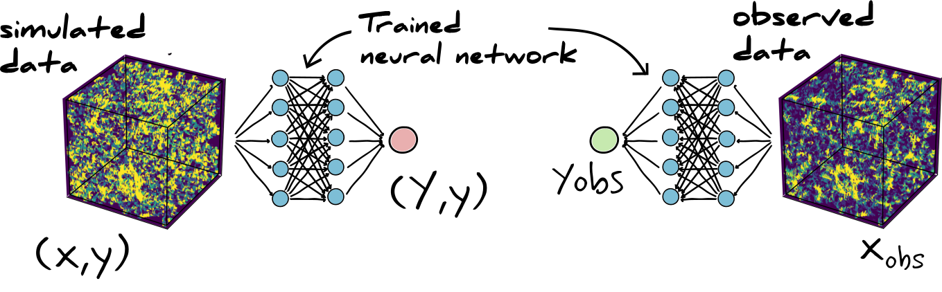
Information maximising neural networks
(Charnock, Lavaux and Wandelt 2018)
Completely different use for network (not modelling)
Find the function which maximises the information about your parameters
- Don't actually care what the network outputs, but we can make them nice, i.e. Gaussianly distributed, etc.
This makes use of the deep learning framework, and the neural network, but for a very different purpose!
Gaussian Fisher information
$$\begin{align*} {\bf F}_{\alpha\beta} &= \left.\left\langle\frac{\partial\ln L(x|y)}{\partial y_\alpha}\frac{\partial\ln L(x|y)}{\partial y_\beta}\right\rangle\right|_{y=y^\textrm{fid}}\\ &=\frac{\partial\mu(y)}{\partial y_\alpha}^T{\bf C}^{-1}\frac{\partial\mu(y)}{\partial y_\beta} \end{align*}$$If we do not know the likelihood $L(x|y)$, transform the data using a neural network to get the likelihood $L(z|y,w,a)$ , where $z=f_{w,a}(x)$
Then maximise $\ln\det{\bf F}_{\alpha\beta}$ where
$${\bf F}_{\alpha\beta} = \frac{\partial\mu(f_{w,a}(x(y)))}{\partial y_\alpha}^T{\bf C}(f_{w,a}(x(y)))^{-1}\frac{\partial\mu(f_{w,a}(x(y)))}{\partial y_\beta}$$Calculate the mean of the derivative of the network outputs with respect to the parameters, $\displaystyle \frac{\partial\mu(f_{w,a}(x(y)))}{\partial y_\alpha}$
Calculate the covariance of the network outputs with respect to the parameters, ${\bf C}(f_{w,a}(x(y)))$
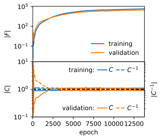
We also want to set the scale of the summaries which we can do with a regulariser (which is arbitrary) like $$\Lambda_2 = \|{\bf C}(f_{w,a}(x(y)))-\mathbb{I}\|+\|{\bf C}(f_{w,a}(x(y)))-\mathbb{I}\|$$
This is all very easy to do using modern frameworks
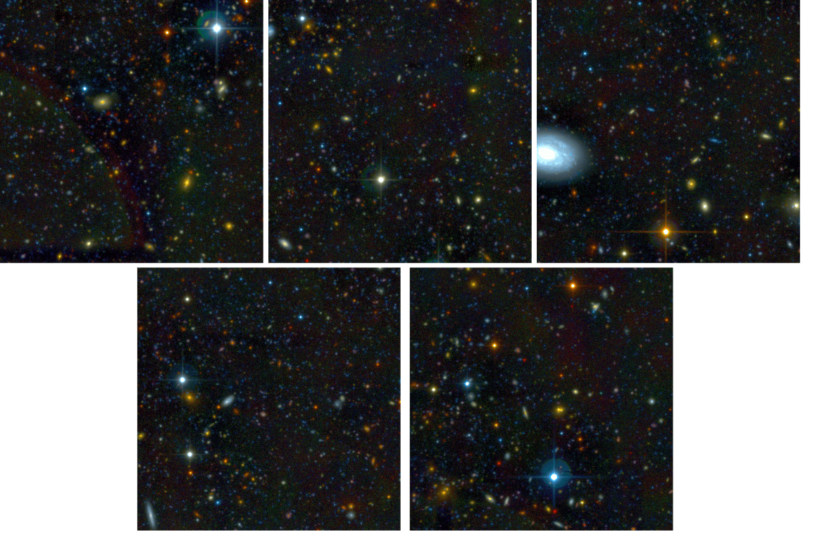
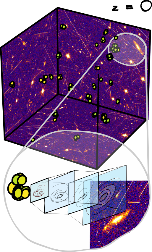
Do not know the likelihood for such a field
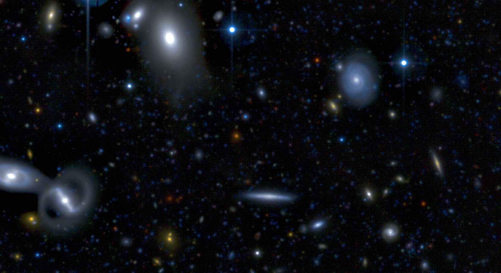
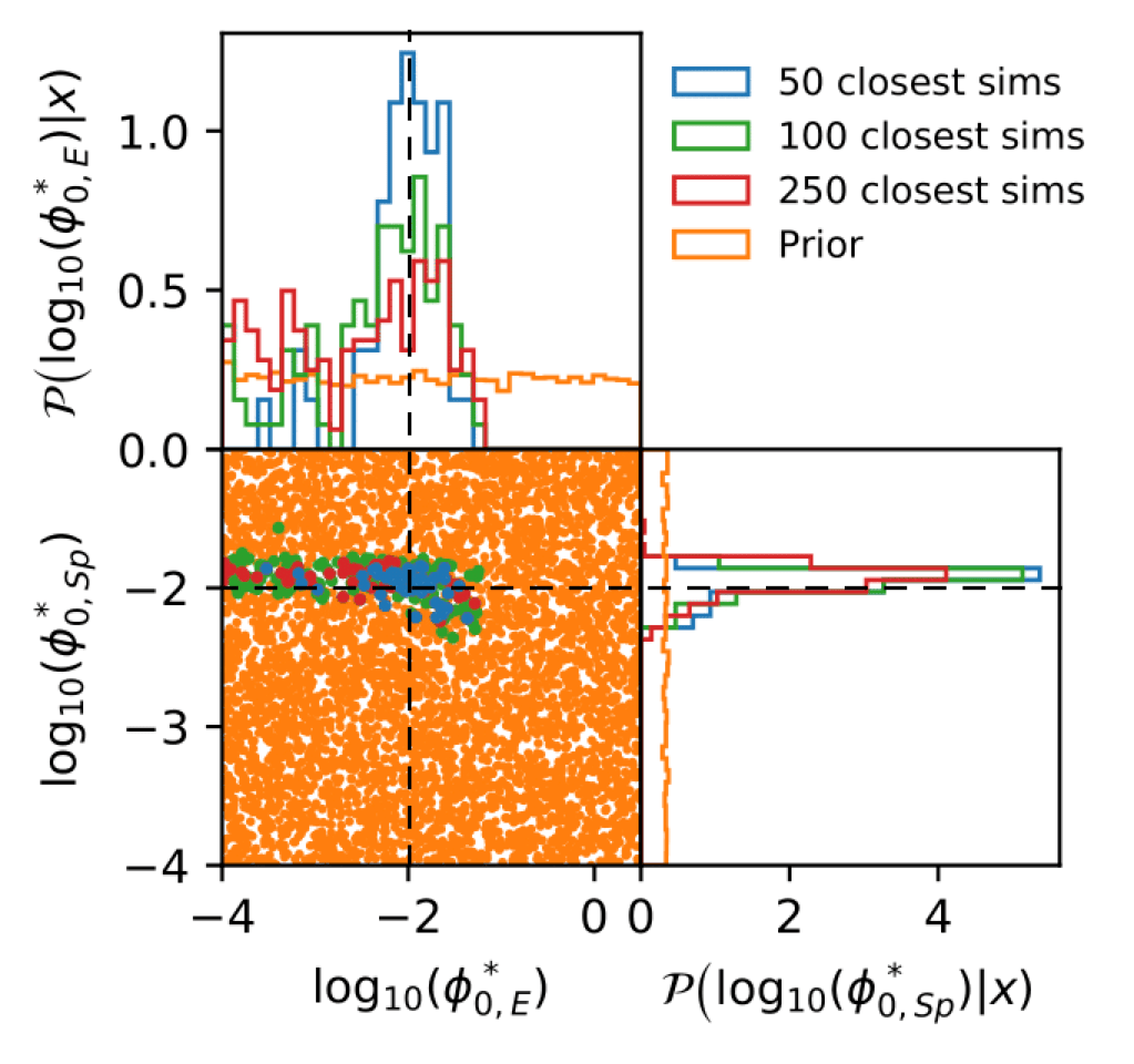
Train IMNN to extract information from such images about the density of spirals and the density of ellipticals
Conclusions
Machine learning is great - but its rubbish at doing science
It can be, however, be used to enable science:
- to speed up analyses or give indications of where to build models
- to build agnostic data models which can be marginalised out
- for super-informative compression to increase the statistical power of current inference methods